Gradient Boosting

Gradient Boosting Machines (GBMs)

GBMs are extremely popular, successful across many domains and one of the leading methods for winning Kaggle competitions.
GBMs build an ensemble of flat and weak successive trees with each tree learning and improving on the previous.
When combined, these trees produce a powerful “committee” often hard to beat with other algorithms.
The following slides are based on UC Business Analytics R Programming Guide on GBM regression

The idea of GBMs

Many machine learning models are founded on a single predictive model (i.e. linear regression, penalized models, naive bayes, svm).
Other approaches (bagging, random forests) are built on the idea of building an ensemble of models where each individual model predicts the outcome and the ensemble simply averages the predicted values. <!–
The family of boosting methods is based on a different, constructive strategy of ensemble formation. –>
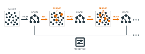
The idea of boosting is to add models to the ensemble sequentially.
At each particular iteration, a new weak, base-learner model is trained with respect to the error of the whole ensemble learnt so far.

Sequential ensemble approach { height=70% }

Advantages of GBMs

Predictive accuracy

GBMs often provide predictive accuracy that cannot be beat.

Flexibility

Optimization on various loss functions possible and several hyperparameter tuning options.

No data pre-processing required

Often works great with categorical and numerical values as is.

Handles missing data

Imputation not required.

Disadvantages of GBMs

GBMs overemphasize outliers

This causes overfitting.
GBMs will continue improving to minimize all errors. Use cross-validation to neutralize.

Computationally expensive

GBMs often require many trees (>1000) which can be time and memory exhaustive.
The high flexibility results in many parameters that interact and influence heavily the behavior of the approach (number of iterations, tree depth, regularization parameters, etc.).
This requires a large grid search during tuning.

Interpretability

GBMs are less interpretable, but this is easily addressed with various tools (variable importance, partial dependence plots, LIME, etc.).

Important concepts

Base-learning models

Boosting is a framework that iteratively improves any weak learning model.
Many gradient boosting applications allow you to “plug in” various classes of weak learners at your disposal.
In practice, boosted algorithms often use decision trees as the base-learner. <!–
Consequently, this tutorial will discuss boosting in the context of regression trees. –>

Training weak models

A weak model has an error rate only slightly better than random guessing.
The idea behind boosting is that each sequential model builds a simple weak model to slightly improve the remaining errors.
Shallow trees represent weak learner - trees with only 1-6 splits.

Benefits of combining many weak models:

Speed: Constructing weak models is computationally cheap.
Accuracy improvement: Weak models allow the algorithm to learn slowly; making minor adjustments in new areas where it does not perform well. In general, statistical approaches that learn slowly tend to perform well.
Avoids overfitting: Making only small incremental improvements with each model in the ensemble allows us to stop the learning process as soon as overfitting has been detected (typically by using cross-validation).

Sequential training with respect to errors

Boosted trees are grown sequentially;
Each tree is grown using information from previously grown trees.
$x \rightarrow$ features and $y \rightarrow$ response:
The basic algorithm for boosted regression trees can be generalized:

1.) Fit a decission tree: $F_1(x)=y$

2.) the next decission tree is fixed to the residuals of the previous: $h_1(x)=y-F_1(x)$

3.) Add this new tree to our algorithm: $F_2(x)=F_1(x)+h_1(x)$

4.) The next decission tree is fixed to the residuals of $h_2(x)=y-F_2(x)$

5.) Add the new tree to the algorithm: $F_3(x)=F_2(x) + h_1(x)$

Continue this process until some mechanism (i.e. cross validation) tells us to stop.

Boosted regression decision stumps as 0-1024 successive trees are added.

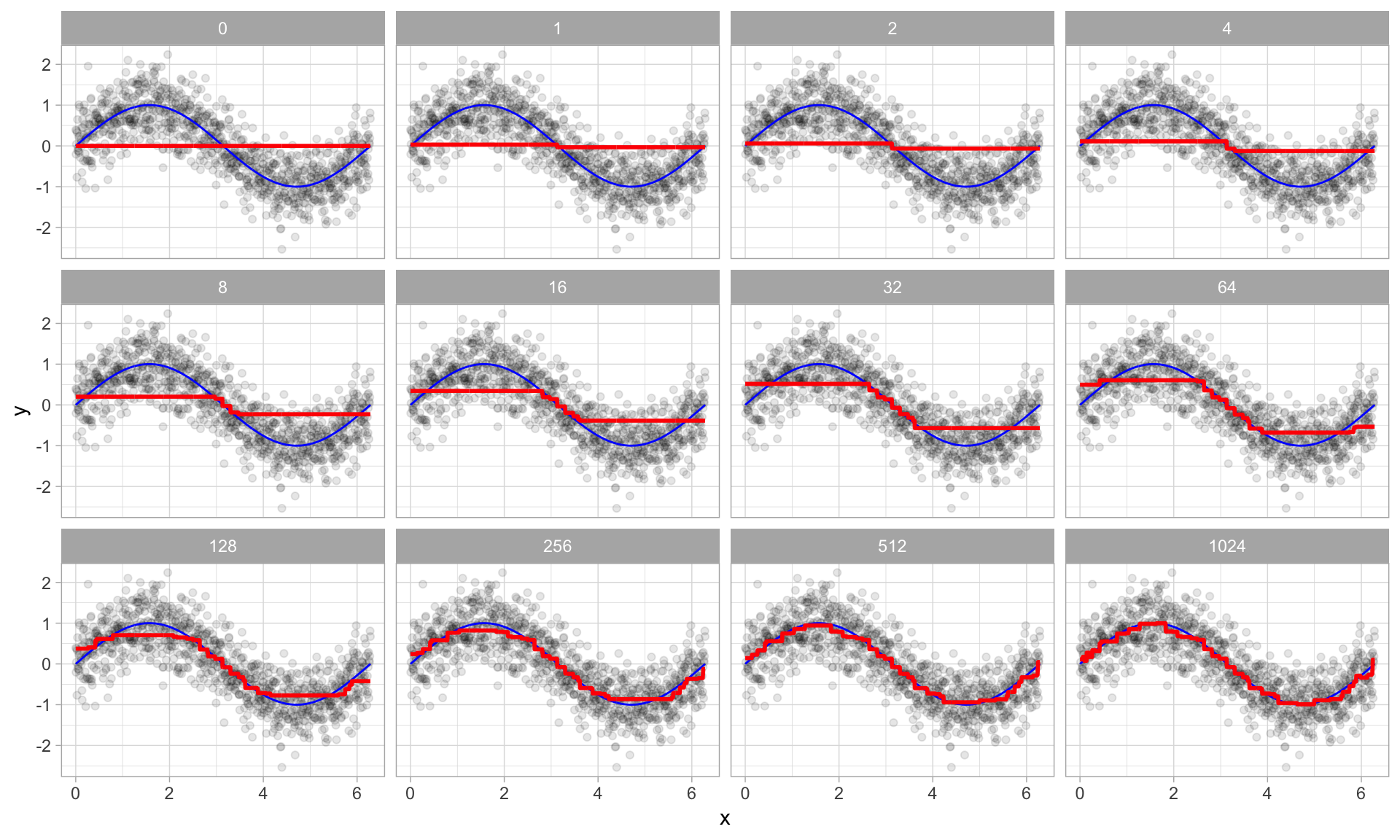
Boosted regression figure - explained

The figure illustrates a single predictor ($x$) that has a true underlying sine wave relationship (blue line) with y along with some irriducible error.
The first tree fit in the series is a single decision stump (i.e., a tree with a single split).
Each following successive decision stump is fit to the previous one’s residuals.
Initially there are large errors, but each additional decision stump in the sequence makes a small improvement in different areas across the feature space where errors still remain.

Loss functions

Many algorithms, including decision trees, focus on minimizing the residuals and emphasize the MSE loss function.
In GBM approach, regression trees are fitted sequentially to minimize the errors. <!–
This minimizes the loss function - mean squared error (MSE). –>
Often we wish to focus on other loss functions such as mean absolute error (MAE)
Or we want to apply the method to a classification problem with a loss function such as deviance.
With gradient boosting machines we can generalize the procedure to loss functions other than MSE. <!–
The name gradient boosting machines come from the fact that this procedure can be generalized to loss functions other than MSE. –>

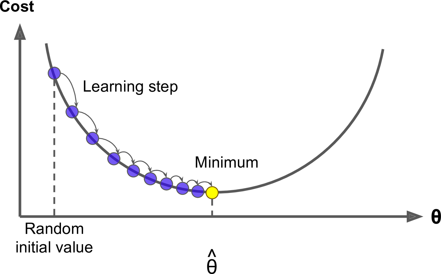
A gradient descent algorithm

Gradient boosting is considered a gradient descent algorithm.
Which is a very generic optimization algorithm capable of finding optimal solutions to a wide range of problems.
The general idea of gradient descent is to tweak parameters iteratively in order to minimize a cost function.

Example

Suppose you are a downhill skier racing against your friend.
A good strategy to beat your friend is to take the path with the steepest slope.
This is exactly what gradient descent does - it measures the local gradient of the loss (cost) function for a given set of parameters ($\Phi$) and takes steps in the direction of the descending gradient.
Once the gradient is zero, we have reached the minimum.

Gradient descent (Geron, 2017).

Gradient descent

Gradient descent can be performed on any loss function that is differentiable.
This allows GBMs to optimize different loss functions as desired
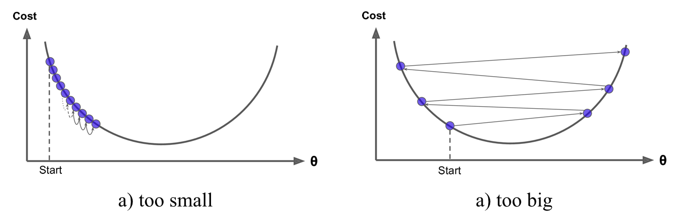
An important parameter in gradient descent is the size of the steps which is determined by the learning rate.
If the learning rate is too small, then the algorithm will take many iterations to find the minimum.
But if the learning rate is too high, you might jump cross the minimum and end up further away than when you started.

Learning rate comparisons (Geron, 2017).

Shape of cost functions

Not all cost functions are convex (bowl shaped).
There may be local minimas, plateaus, and other irregular terrain of the loss function that makes finding the global minimum difficult.
Stochastic gradient descent can help us address this problem.
Stochastic because the method uses randomly selected (or shuffled) samples to evaluate the gradients.
By sampling a fraction of the training observations (typically without replacement) and growing the next tree using that subsample.
This makes the algorithm faster but the stochastic nature of random sampling also adds some random nature in descending the loss function gradient.
Although this randomness does not allow the algorithm to find the absolute global minimum, it can actually help the algorithm jump out of local minima and off plateaus and get near the global minimum.

Tuning GBM

GBMs are highly flexible - many tuning parameters
It is time consuming to find the optimal combination of hyperparameters

Number of trees

GBMs often require many trees;
GBMs can overfit so the goal is to find the optimal number of trees that minimize the loss function of interest with cross validation.

Tuning parameters

Depth of trees

The number $d$ of splits in each tree, which controls the complexity of the boosted ensemble.
Often $d=1$ works well, in which case each tree is a stump consisting of a single split. More commonly, $d$ is greater than 1 but it is unlikely that $d>10$ will be required.

Learning rate

Controls how quickly the algorithm proceeds down the gradient descent.
Smaller values reduce the chance of overfitting but also increases the time to find the optimal fit.
This is also called shrinkage.

Tuning parameters (II)

Subsampling

Controls if a fraction of the available training observations is used.
Using less than 100% of the training observations means you are implementing stochastic gradient descent.
This can help to minimize overfitting and keep from getting stuck in a local minimum or plateau of the loss function gradient.

The necessary packages

library(rsample)      # data splitting 
library(gbm)          # basic implementation
library(xgboost)      # a faster implementation of gbm
library(caret)        # aggregator package - machine learning
library(pdp)          # model visualization
library(ggplot2)      # model visualization
library(lime)         # model visualization

The dataset

Again, we use the Ames housing dataset

ames_data <- AmesHousing::make_ames()

set.seed(123)
ames_split <- initial_split(ames_data,prop=.7)
ames_train <- training(ames_split)
ames_test  <- testing(ames_split)

Package implementation

The most popular implementations of GBM in R:

gbm

The original R implementation of GBMs

xgboost

A fast and efficient gradient boosting framework (C++ backend).

h2o

A powerful java-based interface that provides parallel distributed algorithms and efficient productionalization.

The R-package `gbm`

The gbm R package is an implementation of extensions to Freund and Schapire’s AdaBoost algorithm and Friedman’s gradient boosting machine.

Basic implementation - training function

Two primary training functions are available: gbm::gbm and gbm::gbm.fit.
gbm::gbm uses the formula interface to specify the model
gbm::gbm.fit requires the separated x and y matrices (more efficient with many variables).

The default settings in gbm include a learning rate (shrinkage) of 0.001.
This is a very small learning rate and typically requires a large number of trees to find the minimum MSE.
gbm uses the default number of 100 trees, which is rarely sufficient.
The default depth of each tree (interaction.depth) is 1, which means we are ensembling a bunch of stumps.
We will use cv.folds to perform a 5 fold cross validation.
The model takes about 90 seconds to run and the results show that the MSE loss function is minimized with 10000 trees.

Train a GBM model

distribution - depends on the response (e.g. bernoulli for binomial)
gaussian is the defaulf value

set.seed(123)
gbm.fit <- gbm(formula = Sale_Price ~ .,distribution="gaussian",
  data = ames_train,n.trees = 10000,interaction.depth = 1,
  shrinkage = 0.001,cv.folds = 5,n.cores = NULL,verbose = FALSE)  

print(gbm.fit) # print results

## gbm(formula = Sale_Price ~ ., distribution = "gaussian", data = ames_train, 
##     n.trees = 10000, interaction.depth = 1, shrinkage = 0.001, 
##     cv.folds = 5, verbose = FALSE, n.cores = NULL)
## A gradient boosted model with gaussian loss function.
## 10000 iterations were performed.
## The best cross-validation iteration was 10000.
## There were 80 predictors of which 45 had non-zero influence.

Exercise

Take some time to dig around in the gbm.fit object to get comfortable with its components.

The output object…

… is a list containing several modelling and results information.
We can access this information with regular indexing;
The minimum CV RMSE is 29133 (this means on average our model is about $29,133 off from the actual sales price) but the plot also illustrates that the CV error is still decreasing at 10,000 trees.

Get MSE

sqrt(min(gbm.fit$cv.error))

## [1] 29133.33

Plot loss function as a result of n trees added to the ensemble

gbm.perf(gbm.fit, method = "cv")

## [1] 10000

Tuning GBMs

The learning rate is increased to take larger steps down the gradient descent,
The number of trees is reduced (since we reduced the learning rate), and increase the depth of each tree.

set.seed(123)
gbm.fit2 <- gbm(formula = Sale_Price ~ .,
  distribution = "gaussian",data = ames_train,
  n.trees = 5000,interaction.depth = 3,shrinkage = 0.1,
  cv.folds = 5,n.cores = NULL,verbose = FALSE)  

# find index for n trees with minimum CV error
min_MSE <- which.min(gbm.fit2$cv.error)
# get MSE and compute RMSE
sqrt(gbm.fit2$cv.error[min_MSE])

## [1] 23112.1

plot loss function as a result of n trees added to the ensemble

Assess the GBM performance:

gbm.perf(gbm.fit2, method = "cv")

## [1] 1260

Grid search

n.minobsinnode is the minimum number of observations allowed in the trees (nr. for terminal nodes is varied)

hyper_grid <- expand.grid(
  shrinkage = c(.01, .1, .3),
  interaction.depth = c(1, 3, 5),
  n.minobsinnode = c(5, 10, 15),
  bag.fraction = c(.65, .8, 1), 
  optimal_trees = 0,# a place to dump results
  min_RMSE = 0                     
)

# total number of combinations
nrow(hyper_grid)

## [1] 81

Randomize data

train.fraction use the first XX% of the data so its important to randomize the rows in case there is any logic ordering (i.e. ordered by neighborhood).

random_index <- sample(1:nrow(ames_train), nrow(ames_train))
random_ames_train <- ames_train[random_index, ]

Grid search - loop over hyperparameter grid

for(i in 1:nrow(hyper_grid)) {
  set.seed(123)
  gbm.tune <- gbm(
    formula = Sale_Price ~ .,distribution = "gaussian",
    data = random_ames_train,n.trees = 5000,
    interaction.depth = hyper_grid$interaction.depth[i],
    shrinkage = hyper_grid$shrinkage[i],
    n.minobsinnode = hyper_grid$n.minobsinnode[i],
    bag.fraction = hyper_grid$bag.fraction[i],
    train.fraction = .75,n.cores = NULL,verbose = FALSE
  )
  # add min training error and trees to grid
  hyper_grid$optimal_trees[i] <- which.min(gbm.tune$valid.error)
  hyper_grid$min_RMSE[i] <- sqrt(min(gbm.tune$valid.error))
}

The top 10 values

hyper_grid %>% 
  dplyr::arrange(min_RMSE) %>%
  head(10)

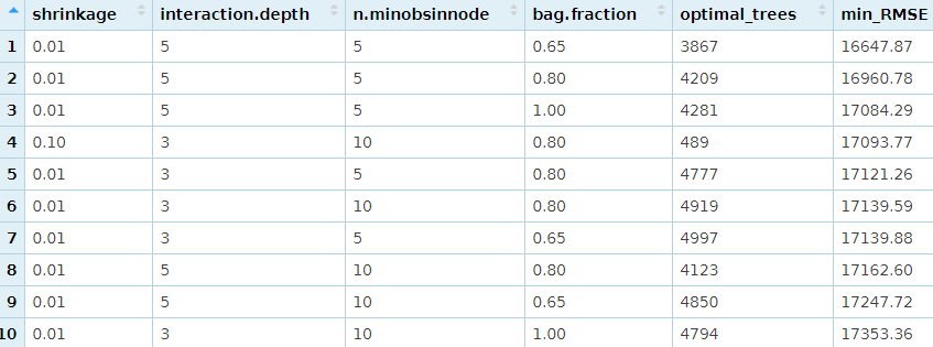
Loop through hyperparameter combinations

We loop through each hyperparameter combination (5,000 trees).
To speed up the tuning process, instead of performing 5-fold CV we train on 75% of the training observations and evaluate performance on the remaining 25%.

The top model has better performance than our previously fitted model, with a RMSE nearly $3,000 and lower.

A look at the top 10 models:

None of the top models used a learning rate of 0.3; small incremental steps down the gradient descent work best,
None of the top models used stumps (interaction.depth = 1); there are likely some important interactions that the deeper trees are able to capture.
Adding a stochastic component with bag.fraction < 1 seems to help; there may be some local minimas in our loss function gradient,

Refine the search - adjust the grid

# modify hyperparameter grid
hyper_grid <- expand.grid(
  shrinkage = c(.01, .05, .1),
  interaction.depth = c(3, 5, 7),
  n.minobsinnode = c(5, 7, 10),
  bag.fraction = c(.65, .8, 1), 
  optimal_trees = 0,# a place to dump results
  min_RMSE = 0# a place to dump results
)

# total number of combinations
nrow(hyper_grid)

## [1] 81

The final model

set.seed(123)
# train GBM model
gbm.fit.final <- gbm(formula = Sale_Price ~ .,
  distribution = "gaussian",data = ames_train,
  n.trees = 483,interaction.depth = 5,
  shrinkage = 0.1,n.minobsinnode = 5,
  bag.fraction = .65,train.fraction = 1,
  n.cores = NULL, # will use all cores by default
  verbose = FALSE)  

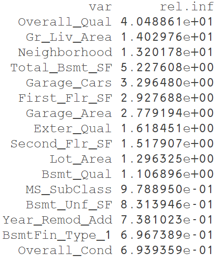
Visualizing - Variable importance

cBars allows you to adjust the number of variables to show

summary(gbm.fit.final,cBars = 10,
  # also can use permutation.test.gbm
  method = relative.influence,las = 2)

##                                   var      rel.inf
## Overall_Qual             Overall_Qual 4.048861e+01
## Gr_Liv_Area               Gr_Liv_Area 1.402976e+01
## Neighborhood             Neighborhood 1.320178e+01
## Total_Bsmt_SF           Total_Bsmt_SF 5.227608e+00
## Garage_Cars               Garage_Cars 3.296480e+00
## First_Flr_SF             First_Flr_SF 2.927688e+00
## Garage_Area               Garage_Area 2.779194e+00
## Exter_Qual                 Exter_Qual 1.618451e+00
## Second_Flr_SF           Second_Flr_SF 1.517907e+00
## Lot_Area                     Lot_Area 1.296325e+00
## Bsmt_Qual                   Bsmt_Qual 1.106896e+00
## MS_SubClass               MS_SubClass 9.788950e-01
## Bsmt_Unf_SF               Bsmt_Unf_SF 8.313946e-01
## Year_Remod_Add         Year_Remod_Add 7.381023e-01
## BsmtFin_Type_1         BsmtFin_Type_1 6.967389e-01
## Overall_Cond             Overall_Cond 6.939359e-01
## Kitchen_Qual             Kitchen_Qual 6.649051e-01
## Garage_Type               Garage_Type 5.727906e-01
## Fireplace_Qu             Fireplace_Qu 5.281111e-01
## Bsmt_Exposure           Bsmt_Exposure 4.601763e-01
## Sale_Type                   Sale_Type 4.063181e-01
## Exterior_1st             Exterior_1st 3.889487e-01
## Open_Porch_SF           Open_Porch_SF 3.797533e-01
## Sale_Condition         Sale_Condition 3.771138e-01
## Exterior_2nd             Exterior_2nd 3.482380e-01
## Year_Built                 Year_Built 3.289944e-01
## Full_Bath                   Full_Bath 3.070894e-01
## Screen_Porch             Screen_Porch 2.907584e-01
## Fireplaces                 Fireplaces 2.906831e-01
## Bsmt_Full_Bath         Bsmt_Full_Bath 2.890666e-01
## Wood_Deck_SF             Wood_Deck_SF 2.448412e-01
## Longitude                   Longitude 2.249308e-01
## Central_Air               Central_Air 2.232338e-01
## Condition_1               Condition_1 1.867403e-01
## Latitude                     Latitude 1.650208e-01
## Lot_Frontage             Lot_Frontage 1.488962e-01
## Heating_QC                 Heating_QC 1.456177e-01
## Mo_Sold                       Mo_Sold 1.406729e-01
## TotRms_AbvGrd           TotRms_AbvGrd 1.162828e-01
## Functional                 Functional 1.118959e-01
## Mas_Vnr_Area             Mas_Vnr_Area 1.005664e-01
## Paved_Drive               Paved_Drive 9.346526e-02
## Land_Contour             Land_Contour 9.026977e-02
## Enclosed_Porch         Enclosed_Porch 7.512751e-02
## Garage_Cond               Garage_Cond 7.143649e-02
## Lot_Config                 Lot_Config 6.355982e-02
## Year_Sold                   Year_Sold 6.198938e-02
## Bedroom_AbvGr           Bedroom_AbvGr 6.146463e-02
## Mas_Vnr_Type             Mas_Vnr_Type 5.820946e-02
## Roof_Style                 Roof_Style 5.682478e-02
## Roof_Matl                   Roof_Matl 4.948087e-02
## Alley                           Alley 4.279173e-02
## BsmtFin_Type_2         BsmtFin_Type_2 3.482743e-02
## Low_Qual_Fin_SF       Low_Qual_Fin_SF 3.427532e-02
## Garage_Qual               Garage_Qual 3.136598e-02
## Foundation                 Foundation 2.803887e-02
## Bsmt_Cond                   Bsmt_Cond 2.768063e-02
## Condition_2               Condition_2 2.751263e-02
## Bsmt_Half_Bath         Bsmt_Half_Bath 2.650291e-02
## MS_Zoning                   MS_Zoning 2.346874e-02
## Pool_QC                       Pool_QC 2.211997e-02
## Half_Bath                   Half_Bath 2.148830e-02
## Three_season_porch Three_season_porch 1.833322e-02
## BsmtFin_SF_2             BsmtFin_SF_2 1.774457e-02
## Garage_Finish           Garage_Finish 1.407325e-02
## Fence                           Fence 1.188101e-02
## House_Style               House_Style 1.105981e-02
## Exter_Cond                 Exter_Cond 1.061516e-02
## Misc_Val                     Misc_Val 7.996187e-03
## Street                         Street 7.460435e-03
## Land_Slope                 Land_Slope 6.847183e-03
## Lot_Shape                   Lot_Shape 6.681489e-03
## Electrical                 Electrical 5.498046e-03
## BsmtFin_SF_1             BsmtFin_SF_1 4.149129e-03
## Pool_Area                   Pool_Area 3.622225e-03
## Misc_Feature             Misc_Feature 7.232842e-04
## Utilities                   Utilities 0.000000e+00
## Bldg_Type                   Bldg_Type 0.000000e+00
## Heating                       Heating 0.000000e+00
## Kitchen_AbvGr           Kitchen_AbvGr 0.000000e+00

Variable importance

Partial dependence plots

PDPs show the marginal effect one or two features have on the predicted outcome.

The following PDP plot displays the average change in predicted sales price as we vary Gr_Liv_Area while holding all other variables constant. <!–
This is done by holding all variables constant for each observation in our training data set but then apply the unique values of Gr_Liv_Area for each observation. –>
We then average the sale price across all the observations.
This PDP illustrates how the predicted sales price increases as the square footage of the ground floor in a house increases.

Partial dependence plot - `Gr_Liv_Area`

gbm.fit.final %>% partial(pred.var = "Gr_Liv_Area", 
          n.trees = gbm.fit.final$n.trees, 
          grid.resolution = 100) %>%
  autoplot(rug = TRUE, train = ames_train) +
  scale_y_continuous(labels = scales::dollar)

Partial dependence plot

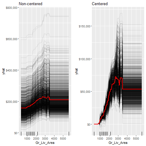
Individual Conditional Expectation (ICE) curves …

… are an extension of PDP plots but the change in the predicted response variable is plotted as we vary each predictor variable. <!–
Below shows the regular ICE curve plot (left) and the centered ICE curves (right). –>
When the curves have a wide range of intercepts and are consequently “stacked” on each other, heterogeneity in the response variable values due to marginal changes in the predictor variable of interest can be difficult to discern.
The centered ICE can help draw these inferences out and can highlight any strong heterogeneity in our results.
The results show that most observations follow a common trend as Gr_Liv_Area increases;
the centered ICE plot highlights a few observations that deviate from the common trend.

Non centered ICE curve

ice1 <- gbm.fit.final %>%
  partial(
    pred.var = "Gr_Liv_Area", 
    n.trees = gbm.fit.final$n.trees, 
    grid.resolution = 100,
    ice = TRUE
    ) %>%
  autoplot(rug = TRUE, train = ames_train, alpha = .1) +
  ggtitle("Non-centered") +
  scale_y_continuous(labels = scales::dollar)

Centered ICE curve

ice2 <- gbm.fit.final %>%
  partial(
    pred.var = "Gr_Liv_Area", 
    n.trees = gbm.fit.final$n.trees, 
    grid.resolution = 100,
    ice = TRUE
    ) %>%
  autoplot(rug = TRUE, train = ames_train, alpha = .1, 
           center = TRUE) +  ggtitle("Centered") +
  scale_y_continuous(labels = scales::dollar)

Non centered and centered ice curve

gridExtra::grid.arrange(ice1, ice2, nrow = 1)

{height=80%}

Local Interpretable Model-Agnostic Explanations – (LIME)

LIME is a newer procedure for understanding why a prediction resulted in a given value for a single observation.
To use the lime package on a gbm model we need to define model type and prediction methods.

model_type.gbm <- function(x, ...) {
  return("regression")
}

predict_model.gbm <- function(x, newdata, ...) {
  pred <- predict(x, newdata, n.trees = x$n.trees)
  return(as.data.frame(pred))
}

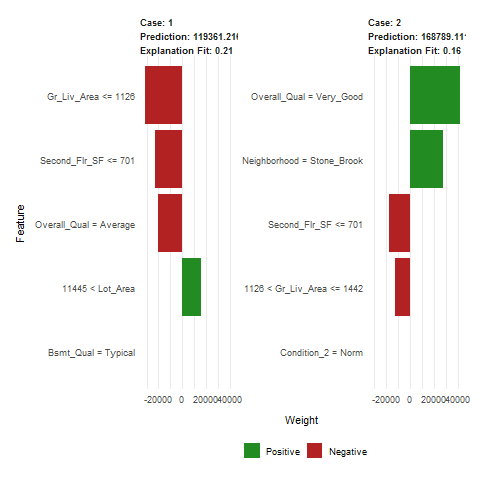
Applying LIME

The results show the predicted value (Case 1: 118K Dollar, Case 2: 161K Dollar), local model fit (both are relatively poor), and the most influential variables driving the predicted value for each observation.

# get a few observations to perform local interpretation on
local_obs <- ames_test[1:2, ]

# apply LIME
explainer <- lime(ames_train, gbm.fit.final)
explanation <- explain(local_obs, explainer, n_features = 5)

LIME plot

plot_features(explanation)

Predicting

If you have decided on a final model you’ll likely want to use the model to predict on new observations.
Like most models, we simply use the predict function; we also need to supply the number of trees to use (see ?predict.gbm for details).
The RMSE for the test set is very close to the RMSE we obtained on our best gbm model.

# predict values for test data
pred <- predict(gbm.fit.final, n.trees = gbm.fit.final$n.trees, 
                ames_test)

# results
caret::RMSE(pred, ames_test$Sale_Price)

## [1] 21533.65

`xgboost`

The xgboost R package provides an R API to “Extreme Gradient Boosting”, which is an efficient implementation of gradient boosting framework (approx. 10x faster than gbm).
The xgboost/demo repository provides a wealth of information. <!– You can also find a fairly comprehensive parameter tuning guide here.

https://www.analyticsvidhya.com/blog/2016/03/complete-guide-parameter-tuning-xgboost-with-codes-python/ –> <!–

The xgboost package has been quite popular and successful on Kaggle for data mining competitions. –>

Features include:

Provides built-in k-fold cross-validation -Stochastic GBM with column and row sampling (per split and per tree) for better generalization.
Includes efficient linear model solver and tree learning algorithms.
Parallel computation on a single machine.
Supports various objective functions, including regression, classification and ranking.
The package is made to be extensible, so that users are also allowed to define their own objectives easily.
Apache 2.0 License.

Basic implementation

XGBoost only works with matrices that contain all numeric variables; consequently, we need to hot encode our data. There are different ways to do this in R (i.e. Matrix::sparse.model.matrix, caret::dummyVars) but here we will use the vtreat package.
vtreat is a robust package for data prep and helps to eliminate problems caused by missing values, novel categorical levels that appear in future data sets that were not in the training data, etc. vtreat is not very intuitive.

Application of `vtreat` to one-hot encode the training and testing data sets.

# variable names
features <- setdiff(names(ames_train), "Sale_Price")
# Create the treatment plan from the training data
treatplan <- vtreat::designTreatmentsZ(ames_train, features, 
                                       verbose = FALSE)

# Get the "clean" variable names from the scoreFrame
new_vars <- treatplan %>%
  magrittr::use_series(scoreFrame) %>%        
  dplyr::filter(code %in% c("clean", "lev")) %>% 
  magrittr::use_series(varName)     

# Prepare the training data
features_train <- vtreat::prepare(treatplan, ames_train, 
                varRestriction = new_vars) %>% as.matrix()
response_train <- ames_train$Sale_Price

Prepare the test data

features_test <- vtreat::prepare(treatplan, ames_test, 
                varRestriction = new_vars) %>% as.matrix()
response_test <- ames_test$Sale_Price

dimensions of one-hot encoded data

dim(features_train)

## [1] 2051  343

dim(features_test)

## [1] 879 343

`xgboost` - training functions

xgboost provides different training functions (i.e. xgb.train which is just a wrapper for xgboost).
To train an XGBoost we typically want to use xgb.cv, which incorporates cross-validation. The following trains a basic 5-fold cross validated XGBoost model with 1,000 trees. There are many parameters available in xgb.cv but the ones used in this tutorial include the following default values:
learning rate ($\eta$): 0.3
tree depth (max_depth): 6
minimum node size (min_child_weight): 1
percent of training data to sample for each tree (subsample –> equivalent to gbm’s bag.fraction): 100%

Extreme gradient boosting for regression models

set.seed(123)
xgb.fit1 <- xgb.cv(
  data = features_train,
  label = response_train,
  nrounds = 1000,  nfold = 5,
  objective = "reg:linear",  # for regression models
  verbose = 0               # silent,
)

get number of trees that minimize error

The xgb.fit1 object contains lots of good information.
In particular we can assess the xgb.fit1$evaluation_log to identify the minimum RMSE and the optimal number of trees for both the training data and the cross-validated error.
The training error continues to decrease to 924 trees where the RMSE nearly reaches zero;
The cross validated error reaches a minimum RMSE of 27,337 with only 60 trees.

xgb.fit1$evaluation_log %>%
  dplyr::summarise(
  ntrees.train=which(train_rmse_mean==min(train_rmse_mean))[1],
  rmse.train= min(train_rmse_mean),
  ntrees.test=which(test_rmse_mean==min(test_rmse_mean))[1],
  rmse.test   = min(test_rmse_mean)
)

##   ntrees.train rmse.train ntrees.test rmse.test
## 1          924  0.0483002          60  27337.79

Plot error vs number trees

ggplot(xgb.fit1$evaluation_log) +
  geom_line(aes(iter, train_rmse_mean), color = "red") +
  geom_line(aes(iter, test_rmse_mean), color = "blue")

Early stopping

A nice feature provided by xgb.cv is early stopping.
This allows us to tell the function to stop running if the cross validated error does not improve for n continuous trees.
E.g., the above model could be re-run with the following where we tell it stop if we see no improvement for 10 consecutive trees. This feature will help us speed up the tuning process.

set.seed(123)
xgb.fit2 <- xgb.cv(data = features_train,
  label = response_train,
  nrounds = 1000,  nfold = 5,
  objective = "reg:linear",  # for regression models
  verbose = 0,               # silent,
  # stop if no improvement for 10 consecutive trees
  early_stopping_rounds = 10)

plot error vs number trees

ggplot(xgb.fit2$evaluation_log) +
  geom_line(aes(iter, train_rmse_mean), color = "red") +
  geom_line(aes(iter, test_rmse_mean), color = "blue")

Tuning

To tune the XGBoost model we pass parameters as a list object to the params argument. The most common parameters include:
eta:controls- the learning rate
max_depth: tree depth
min_child_weight: minimum number of observations required in each terminal node
subsample: percent of training data to sample for each tree
colsample_bytrees: percent of columns to sample from for each tree
E.g. to specify specific values for these parameters we would extend the above model with the following parameters.

create parameter list

  params <- list(
    eta = .1,
    max_depth = 5,
    min_child_weight = 2,
    subsample = .8,
    colsample_bytree = .9
  )

To perform a large search grid,…

we can follow the same procedure we did with gbm.
We create our hyperparameter search grid along with columns to dump our results in.
Here, we have a pretty large search grid consisting of 576 different hyperparameter combinations to model.

# create hyperparameter grid
hyper_grid <- expand.grid(
  eta = c(.01, .05, .1, .3),
  max_depth = c(1, 3, 5, 7),
  min_child_weight = c(1, 3, 5, 7),
  subsample = c(.65, .8, 1), 
  colsample_bytree = c(.8, .9, 1),
  optimal_trees = 0,# a place to dump results
  min_RMSE = 0# a place to dump results
)

nrow(hyper_grid)

## [1] 576

train model

set.seed(123)
xgb.fit3 <- xgb.cv(
  params = params,
  data = features_train,
  label = response_train,
  nrounds = 1000,
  nfold = 5,
  objective = "reg:linear",  # for regression models
  verbose = 0,               # silent,
  # stop if no improvement for 10 consecutive trees
  early_stopping_rounds = 10 
)

assess results

xgb.fit3$evaluation_log %>%
  dplyr::summarise(
    ntrees.train=which(train_rmse_mean==min(train_rmse_mean))[1],
    rmse.train= min(train_rmse_mean),
    ntrees.test= which(test_rmse_mean==min(test_rmse_mean))[1],
    rmse.test= min(test_rmse_mean)
  )

##   ntrees.train rmse.train ntrees.test rmse.test
## 1          211   5222.229         201  24411.64

Loop through a `XGBoost` model

We apply the same in the loop and apply a XGBoost model for each hyperparameter combination and dump the results in the hyper_grid data frame.

Important note:

If you plan to run this code be prepared to run it before going out to eat or going to bed as it the full search grid took 6 hours to run!

Grid search

for(i in 1:nrow(hyper_grid)) {
  params <- list(# create parameter list
    eta = hyper_grid$eta[i],max_depth = hyper_grid$max_depth[i],
    min_child_weight = hyper_grid$min_child_weight[i],
    subsample = hyper_grid$subsample[i],
    colsample_bytree = hyper_grid$colsample_bytree[i])
  set.seed(123)
  xgb.tune <- xgb.cv(params = params,data = features_train,
  label = response_train,nrounds=5000,nfold=5,objective = "reg:linear",
  #stop if no improvement for 10 consecutive trees
    verbose = 0,early_stopping_rounds = 10 )
  # add min training error and trees to grid
  hyper_grid$optimal_trees[i]<-which.min(
    xgb.tune$evaluation_log$test_rmse_mean)
  hyper_grid$min_RMSE[i] <- min(
    xgb.tune$evaluation_log$test_rmse_mean)
}

Result - top 10 models

hyper_grid %>%
  dplyr::arrange(min_RMSE) %>%
  head(10)

##     eta max_depth min_child_weight subsample colsample_bytree
## 1  0.01         1                1      0.65              0.8
## 2  0.05         1                1      0.65              0.8
## 3  0.10         1                1      0.65              0.8
## 4  0.30         1                1      0.65              0.8
## 5  0.01         3                1      0.65              0.8
## 6  0.05         3                1      0.65              0.8
## 7  0.10         3                1      0.65              0.8
## 8  0.30         3                1      0.65              0.8
## 9  0.01         5                1      0.65              0.8
## 10 0.05         5                1      0.65              0.8
##    optimal_trees min_RMSE
## 1              0        0
## 2              0        0
## 3              0        0
## 4              0        0
## 5              0        0
## 6              0        0
## 7              0        0
## 8              0        0
## 9              0        0
## 10             0        0

The top model

After assessing the results you would likely perform a few more grid searches to hone in on the parameters that appear to influence the model the most. <!–
Here is a link to a great blog post that discusses a strategic approach to tuning with xgboost. –>
We’ll just assume the top model in the above search is the globally optimal model. Once you’ve found the optimal model, we can fit our final model with xgb.train.

# parameter list
params <- list(
  eta = 0.01,
  max_depth = 5,
  min_child_weight = 5,
  subsample = 0.65,
  colsample_bytree = 1
)

Train final model

xgb.fit.final <- xgboost(
  params = params,
  data = features_train,
  label = response_train,
  nrounds = 1576,
  objective = "reg:linear",
  verbose = 0
)

Input types for `xgboost`

Input type: xgboost takes several types of input data:

Dense Matrix: R’s dense matrix, i.e. matrix ;
Sparse Matrix: R’s sparse matrix, i.e. Matrix::dgCMatrix ;
Data File: local data files ;
xgb.DMatrix: its own class (recommended).

get information

We get information on an xgb.DMatrix object with getinfo

Visualizing

Variable importance

xgboost provides built-in variable importance plotting. First, you need to create the importance matrix with xgb.importance and then feed this matrix into xgb.plot.importance. There are 3 variable importance measure:

Gain: the relative contribution of the corresponding feature to the model calculated by taking each feature’s contribution for each tree in the model. This is synonymous with gbm’s relative.influence.
Cover: the relative number of observations related to this feature. For example, if you have 100 observations, 4 features and 3 trees, and suppose feature1 is used to decide the leaf node for 10, 5, and 2 observations in tree1, tree2 and tree3 respectively; then the metric will count cover for this feature as 10+5+2 = 17 observations. This will be calculated for all the 4 features and the cover will be 17 expressed as a percentage for all features’ cover metrics.

create importance matrix

Frequency: the percentage representing the relative number of times a particular feature occurs in the trees of the model. In the above example, if feature1 occurred in 2 splits, 1 split and 3 splits in each of tree1, tree2 and tree3; then the weightage for feature1 will be 2+1+3 = 6. The frequency for feature1 is calculated as its percentage weight over weights of all features.

importance_matrix <- xgb.importance(model = xgb.fit.final)

variable importance plot

xgb.plot.importance(importance_matrix, top_n = 10, measure = "Gain")

Variable importance plot

LIME

LIME provides built-in functionality for xgboost objects (see ?model_type).
Just keep in mind that the local observations being analyzed need to be one-hot encoded in the same manner as we prepared the training and test data. Also, when you feed the training data into the lime::lime function be sure that you coerce it from a matrix to a data frame.

# one-hot encode the local observations to be assessed.
local_obs_onehot <- vtreat::prepare(treatplan, local_obs, 
                                    varRestriction = new_vars)

# apply LIME
explainer <- lime(data.frame(features_train), xgb.fit.final)
explanation <- explain(local_obs_onehot, explainer, 
                       n_features = 5)

Plot the features

plot_features(explanation)

Predicting on new observations

unlike GBM we do not need to provide the number of trees. Our test set RMSE is only about $600 different than that produced by our gbm model.

# predict values for test data
pred <- predict(xgb.fit.final, features_test)

# results
caret::RMSE(pred, response_test)

## [1] 21898

## [1] 21319.3

Links and Resources - Boosting

Resources

Geron (2017) - Hands-On Machine Learning with Scikit-Learn and TensorFlow: Concepts, Tools and techniques to build intelligent systems