Random Forests

• Bagging can turn a single tree model with high variance and poor predictive power into a fairly accurate prediction function.
• But bagging suffers from tree correlation, which reduces the overall performance of the model.
• Random forests are a modification of bagging that builds a large collection of de-correlated trees
• It is a very popular out-of-the-box learning algorithm that enjoys good predictive performance.

Extending the bagging technique

• Bagging introduces a random component in to the tree building process
• The trees in bagging are not completely independent of each other since all the original predictors are considered at every split of every tree.
• Trees from different bootstrap samples have similar structure to each other (especially at the top of the tree) due to underlying relationships.

Similar trees - tree correlation

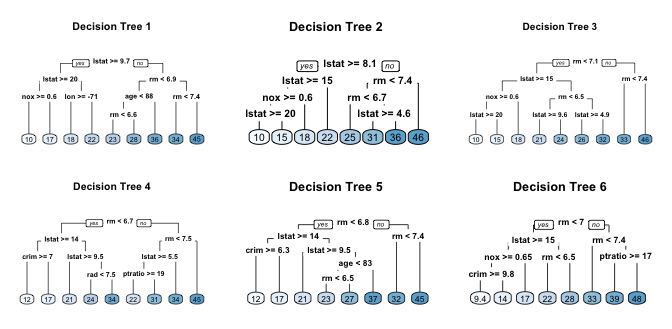
• If we create six decision trees with different bootstrapped samples of the Boston housing data, the top of the trees all have a very similar structure.
• Although there are 15 predictor variables to split on, all six trees have both lstat and rm variables driving the first few splits.

Tree correlation

• Tree correlation prevents bagging from optimally reducing variance of the predictive values.
• To reduce variance further, we need to minimize the amount of correlation between the trees.
• This can be achieved by injecting more randomness into the tree-growing process.

Random forests achieve this in two ways:

1) Bootstrap:

• Similar to bagging, each tree is grown to a bootstrap resampled data set, which makes them different and decorrelates them.

2) Split-variable randomization:

• For every split, the search for the split variable is limited to a random subset of $m$ of the $p$ variables.
• For regression trees, typical default values are $m=p/3$ (tuning parameter).
• When $m=p$, the randomization is limited (only step 1) and is the same as bagging.

Basic algorithm

The basic algorithm for a regression random forest can be generalized:

1.  Given training data set
2.  Select number of trees to build (ntrees)
3.  for i = 1 to ntrees do
4.  |  Generate a bootstrap sample of the original data
5.  |  Grow a regression tree to the bootstrapped data
6.  |  for each split do
7.  |  | Select m variables at random from all p variables
8.  |  | Pick the best variable/split-point among the m
9.  |  | Split the node into two child nodes
10. |  end
11. | Use tree model stopping criteria to determine: tree complete 
12. end

The algorithm randomly selects a bootstrap sample to train and predictors to use at each split.

Characteristics

• Since bootstrap samples and features are selected randomly at each split, we create a more diverse set of trees, which tends to lessen tree correlation beyond bagged trees and often dramatically increase predictive power. <!–
• random forests have the least variability in their prediction accuracy when tuning. –>

out-of-bag error

• Similar to bagging, a natural benefit of the bootstrap resampling process is that random forests have an out-of-bag (OOB) sample that provides an efficient and reasonable approximation of the test error.
• This provides a built-in validation set without any extra work, and you do not need to sacrifice any of your training data to use for validation.
• We are more efficient identifying the number of trees required to stablize the error rate <!– during tuning;

Out-of-bag error vs. validation error

• Some difference between the OOB error and test error are expected.

–>

Preparation - random forests

• The following slides are based on UC Business Analytics R Programming Guide on random forests

library(rsample)      # data splitting 
library(randomForest) # basic implementation
library(ranger)       # a faster implementation of randomForest
# an aggregator package for performing many 
# machine learning models
library(caret)        

The Ames housing data

set.seed(123)
ames_data <- AmesHousing::ames_raw

set.seed(123)
ames_split <- rsample::initial_split(ames_data,prop=.7)
ames_train <- rsample::training(ames_split)
ames_test  <- rsample::testing(ames_split)

Basic implementation

• There are over 20 random forest packages in R.
• To demonstrate the basic implementation we use the randomForest package, the oldest and most well known implementation of the random forest algorithm in R.
• As your data set grows in size randomForest does not scale well (although you can parallelize with foreach).
• To explore and compare a variety of tuning parameters we can find more effective packages.
• The package ranger will be presented in the tuning section.

randomForest::randomForest

• randomForest can use the formula or x-y matrix notation.
• Below we apply the default randomForest model using the formal specification.
• The default random forest performs 500 trees and $\dfrac{\text{nr. features}}{3}=26$ randomly selected predictor variables at each split.

set.seed(123)
# default RF model
(m1 <- randomForest(formula = Sale_Price ~ .,data=ames_train))

## 
## Call:
##  randomForest(formula = Sale_Price ~ ., data = ames_train) 
##                Type of random forest: regression
##                      Number of trees: 500
## No. of variables tried at each split: 26
## 
##           Mean of squared residuals: 639516350
##                     % Var explained: 89.7

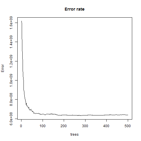
Plotting the model

• The error rate stabalizes with around 100 trees but continues to decrease slowly until around 300 trees.

plot(m1,main="Error rate")

{height=65%}

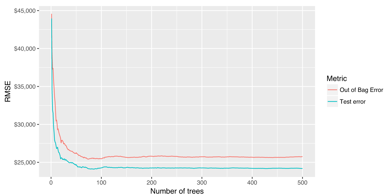
Random forests - out-of-the-box algorithm

• Random forests perform remarkably well with very little tuning.
• We get an RMSE of less than 30K dollar without any tuning.
• This is more than 6K dollar RMSE-reduction compared to a fully-tuned bagging model
• and 4K dollar reduction to to a fully-tuned elastic net model.
• We can still seek improvement by tuning our random forest model.

Tuning Random forests

• Random forests are fairly easy to tune since there are only a handful of tuning parameters.
• First we tune the number of candidate variables to select from at each split.
• A few additional hyperparameters are important.

Tuning parameters (I)

• The following hyperparameter are important (names may differ across packages):

number of trees

• ntree - We want enough trees to stabalize the error but using too many trees is inefficient, esp. for large data sets.

number of variables

• mtry - number of variables as candidates at each split. When mtry=p the model equates to bagging.
• When mtry=1 the split variable is completely random, all variables get a chance but can lead to biased results. Suggestion: start with 5 values evenly spaced across the range from 2 to p.

Tuning parameters (II)

Number of samples

• sampsize - Default value is 63.25% since this is the expected value of unique observations in the bootstrap sample.
• Lower sample sizes can reduce training time but may introduce more bias. Increasing sample size can increase performance but at risk of overfitting - it introduces more variance. <!–
• When tuning this parameter we stay near the 60-80% range. –>

Tuning parameters (III)

minimum number of samples within the terminal nodes:

• nodesize - Controls the complexity of the trees.
• It is the minimum size of terminal nodes.
• Smaller node size allow for deeper, more complex trees
• This is another bias-variance tradeoff where deeper trees introduce more variance (risk of overfitting)
• Shallower trees introduce more bias (risk of not fully capturing unique patters and relatonships in the data).

maximum number of terminal nodes

• maxnodes: A way to control the complexity of the trees.
• More nodes equates to deeper, more complex trees.
• Less nodes result in shallower trees.

Initial tuning with randomForest

• If we just tune the mtry parameter we can use randomForest::tuneRF for a quick and easy tuning assessment. <!–
• tuneRf will start at a value of mtry that you supply and increase by a certain step factor until the OOB error stops improving. –>
• We start with 5 candidate variables (mtryStart=5) and increase by a factor of 2 until the OOB error stops improving by 1 per cent.
• tuneRF requires a separate x y specification.
• The optimal mtry value in this sequence is very close to the default mtry value of $\dfrac{\text{features}}{3}=26$.

features <- setdiff(names(ames_train), "Sale_Price")

set.seed(123)
m2<-tuneRF(x= ames_train[,features],
  y= ames_train$Sale_Price,ntreeTry   = 500,
  mtryStart  = 5,stepFactor = 2,
  improve    = 0.01,trace=FALSE)

Full grid search with ranger

• To perform a larger grid search across several hyperparameters we’ll need to create a grid, loop through each hyperparameter combination and evaluate the model.
• Unfortunately, this is where randomForest becomes quite inefficient since it does not scale well.
• Instead, we can use ranger which is a C++ implementation of Breiman’s random forest algorithm and is over 6 times faster than randomForest.

Assessing the speed

randomForest speed

system.time(
  ames_randomForest <- randomForest(
    formula = Sale_Price ~ ., 
    data    = ames_train, 
    ntree   = 500,
    mtry    = floor(length(features) / 3)
  )
)

#       User      System    elapsed 
#     145.47        0.09      152.48 

ranger speed

system.time(
  ames_ranger <- ranger(formula=Sale_Price ~ ., 
    data      = ames_train,num.trees = 500,
    mtry      = floor(length(features) / 3))
)

##    user  system elapsed 
##    9.13    0.03    3.23

The grid search

• To perform the grid search, we construct our grid of hyperparameters.

# hyperparameter grid search
hyper_grid <- expand.grid(
  mtry       = seq(20, 30, by = 2),
  node_size  = seq(3, 9, by = 2),
  sampe_size = c(.55, .632, .70, .80),
  OOB_RMSE   = 0
)

• We search across 96 different models with varying mtry, minimum node size, and sample size.

nrow(hyper_grid) # total number of combinations

## [1] 96

Loop - hyperparameter combination (I)

• We apply 500 trees since our previous example illustrated that 500 was plenty to achieve a stable error rate.
• We set the random number generator seed. This allows us to consistently sample the same observations for each sample size and make the impact of each change clearer.

for(i in 1:nrow(hyper_grid)) {
  model <- ranger(formula= Sale_Price ~ .,data= ames_train, 
    num.trees       = 500,mtry= hyper_grid$mtry[i],
    min.node.size   = hyper_grid$node_size[i],
    sample.fraction = hyper_grid$sampe_size[i],
    seed            = 123)
    # add OOB error to grid
  hyper_grid$OOB_RMSE[i] <- sqrt(model$prediction.error)
}

The results - samll difference between RMSE

hyper_grid %>% dplyr::arrange(OOB_RMSE) %>% head(10)

##    mtry node_size sampe_size OOB_RMSE
## 1    26         3        0.8 25404.60
## 2    28         3        0.8 25405.92
## 3    28         5        0.8 25459.46
## 4    26         5        0.8 25493.80
## 5    30         3        0.8 25528.26
## 6    22         3        0.7 25552.73
## 7    26         9        0.8 25554.31
## 8    28         7        0.8 25578.45
## 9    20         3        0.8 25581.23
## 10   24         3        0.8 25590.73

• Models with slighly larger sample sizes (70-80 per cent) and deeper trees (3-5 observations in terminal node) perform best.
• We get various mtry values in top 10 - not over influential.

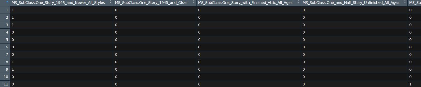
Hyperparameter grid search - categorical variables

• We use one-hot encoding for our categorical variables which produces 353 predictor variables versus the 80 we were using above.

# one-hot encode our categorical variables
(one_hot <- dummyVars(~ ., ames_train, fullRank = FALSE))

## Dummy Variable Object
## 
## Formula: ~.
## 81 variables, 46 factors
## Variables and levels will be separated by '.'
## A less than full rank encoding is used

Make a dataframe of dummy variable object

ames_train_hot<-predict(one_hot,ames_train)%>%as.data.frame()

Hot encoding and hypergrid

# make ranger compatible names
names(ames_train_hot) <- make.names(names(ames_train_hot), 
                                    allow_ = FALSE)
# --> same as above but with increased mtry values
hyper_grid_2 <- expand.grid(
  mtry       = seq(50, 200, by = 25),
  node_size  = seq(3, 9, by = 2),
  sampe_size = c(.55, .632, .70, .80),
  OOB_RMSE  = 0
)

The best model

The best random forest model:

• uses columnar categorical variables
• mtry = 24,
• terminal node size of 5 observations
• sample size of 80%.

How to proceed

• Repeat the model to get a better expectation of error rate.

Random forests with ranger

• The impurity measure is the variance of the responses for regression
• impurity is a measure for heterogeneity - it measures how well the classes are
  <!– https://stats.stackexchange.com/questions/220321/what-is-node-impurity-purity-in-decision-trees-in-plain-english-why-do-we-need

https://people.cs.pitt.edu/~milos/courses/cs2750-Spring03/lectures/class19.pdf –>

OOB_RMSE <- vector(mode = "numeric", length = 100)
for(i in seq_along(OOB_RMSE)) {
  optimal_ranger <- ranger(formula= Sale_Price ~ ., 
    data            = ames_train, 
    num.trees       = 500,
    mtry            = 24,
    min.node.size   = 5,
    sample.fraction = .8,
    importance      = 'impurity')
  OOB_RMSE[i] <- sqrt(optimal_ranger$prediction.error)
}

Variable importance / node impurity

• Node impurity represents how well the trees split the data. There are several impurity measures;

• Gini index, Entropy and misclassification error are options to measure the node impurity

• We set importance = 'impurity', which allows us to assess variable importance.
• Variable importance is measured by recording the decrease in MSE each time a variable is used as a node split in a tree.
• The remaining error left in predictive accuracy after a node split is known as node impurity. <!– https://medium.com/the-artificial-impostor/feature-importance-measures-for-tree-models-part-i-47f187c1a2c3 http://www.cse.msu.edu/~cse802/DecisionTrees.pdf https://www.cs.indiana.edu/~predrag/classes/2017fallb365/ch4.pdf

http://mason.gmu.edu/~jgentle/csi772/16s/L10_CART_16s.pdf

https://stats.stackexchange.com/questions/158583/what-does-node-size-refer-to-in-the-random-forest –>

• A variable that reduces this impurity is considered more imporant than those variables that do not.
• We accumulate the reduction in MSE for each variable across all the trees and the variable with the greatest accumulated impact is considered the more important.

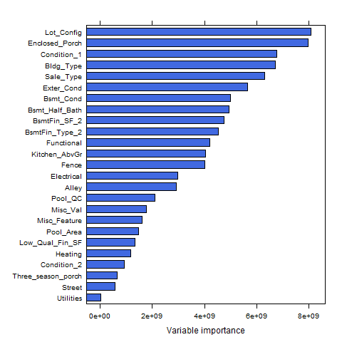
Plot the variable importance

varimp_ranger <- optimal_ranger$variable.importance 

lattice::barchart(sort(varimp_ranger)[1:25],col="royalblue")

• We see that Utilities has the greatest impact in reducing MSE across our trees, followed by names(sort(varimp_ranger))[2], Low_Qual_Fin_SF, etc.

{height=60%}

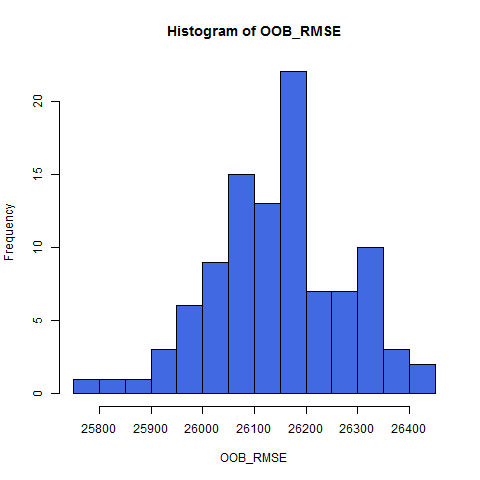
A histogram of OOB RMSE

hist(OOB_RMSE, breaks = 20,col="royalblue")

{height=75%}

Predicting

• With the preferred model we can use the traditional predict function to make predictions on a new data set.
• We can use this for all our model types (randomForest and ranger); although the outputs differ slightly. <!–
• not that the new data for the h2o model needs to be an h2o object. –>

# randomForest
pred_randomForest <- predict(ames_randomForest, ames_test)
head(pred_randomForest)

##        1        2        3        4        5        6 
## 113543.1 185556.4 259258.1 190943.9 179071.0 480952.3

# ranger
pred_ranger <- predict(ames_ranger, ames_test)
head(pred_ranger$predictions)

## [1] 129258.1 186520.7 265628.2 197745.5 175517.6 392691.7

Summary - random forests

• Random forests provide a very powerful out-of-the-box algorithm that often has great predictive accuracy.
• Because of their more simplistic tuning nature and the fact that they require very little, if any, feature pre-processing they are often one of the first go-to algorithms when facing a predictive modeling problem.

Advantages & Disadvantages

Advantages - random forrests

• Typically have very good performance
• Remarkably good “out-of-the box” - very little tuning required
• Built-in validation set - don’t need to sacrifice data for extra validation
• No pre-processing required
• Robust to outliers

Disadvantages - random forrests

• Can become slow on large data sets
• Although accurate, often cannot compete with advanced boosting algorithms
• Less interpretable

Links

These slides are mainly based on

• A UC Business Analytics R Programming Guide - section random forests

• and on the chapter on random forests in the e-book of Brad Boehmke and Brandon Greenwell - Hands-on Machine Learning with R

• Rpubs tutorial - random forests

• Random Forests in R

• Boston Dataset-Tree Family Part-1