Supervised Learning - Regression Trees and Bagging

Tree-Based Models

Trees are good for interpretation because they are simple
Tree based methods involve stratifying or segmenting the predictor space into a number of simple regions. (Hastie and Tibshirani)

But:

These methods do not deliver the best results concerning prediction accuracy.

The Idea

There are many methodologies for constructing regression trees but one of the oldest is the classification and regression tree (CART) approach by Breiman et al. (1984).
Basic regression trees partition a data set into smaller subgroups and then fit a simple constant for each observation in the subgroup.
The partitioning is achieved by successive binary partitions (aka recursive partitioning) based on the different predictors.
The constant to predict is based on the average response values for all observations that fall in that subgroup.

Explanation: decision tree

Decision trees model data as a “tree” of hierarchical branches. They make branches until they reach “leaves” that represent predictions.

[Decission tree on ElitedataScience](https://elitedatascience.com/algorithm-selection)

Example decission trees

Due to their branching structure, decision trees can easily model nonlinear relationships.

Example

For single family homes (larger lots) higher prices,
and for apartments (smaller lots), also higher prices (because here it’s a proxy for urban / rural).

This reversal of correlation is difficult for linear models to capture unless you explicitly add an interaction term

Decision trees can capture this relationship naturally.

Model foundations

This simple example can be generalized
We have a continuous response variable $Y$ and two inputs $X_1$ and $X_2$.
The recursive partitioning results in three regions ($R_1$,$R_2$,$R_3$) where the model predicts $Y$ with a constant $c_m$ for region $R_m$:

$\hat{f} (X) = \sum\limits_{m=1}^3c_mI(X_1,X_2)\in R_m$

How to grow a regression tree - deciding on splits

It is important to realize the partitioning of variables are done in a top-down approach.
A partition performed earlier in the tree will not change based on later partitions.

How are these partions made?

The model begins with the entire data set, $S$, and searches every distinct value of every input variable to find the predictor and split value that partitions the data into two regions ($R_1$ and $R_2$) such that the overall sums of squares error are minimized:

$\text{minimize}\{SSE=\sum\limits_{i\in R_1}(y_i - c_1)^2 + \sum\limits_{i\in R_2} (y_i - c_2)^2 \}$

The best split

Having found the best split, we partition the data into the two resulting regions and repeat the splitting process on each of the two regions.
This process is continued until some stopping criterion is reached.
We typically get a very deep, complex tree that may produce good predictions on the training set, but is likely to overfit the data, leading to poor performance on unseen data.

Regression Trees - preparation

The following slides are based on the UC Business Analytics R Programming Guide on regression trees

library(rsample)     # data splitting 
library(dplyr)       # data wrangling
library(rpart)       # performing regression trees
library(rpart.plot)  # plotting regression trees
library(ipred)       # bagging
library(caret)       # bagging

The Ames Housing data

Again we use the Ames dataset and split it in a test and training dataset

set.seed(123)
ames_data <- AmesHousing::make_ames()
ames_split <- initial_split(ames_data,prop = .7)
ames_train <- training(ames_split)
ames_test  <- testing(ames_split)

Pruning

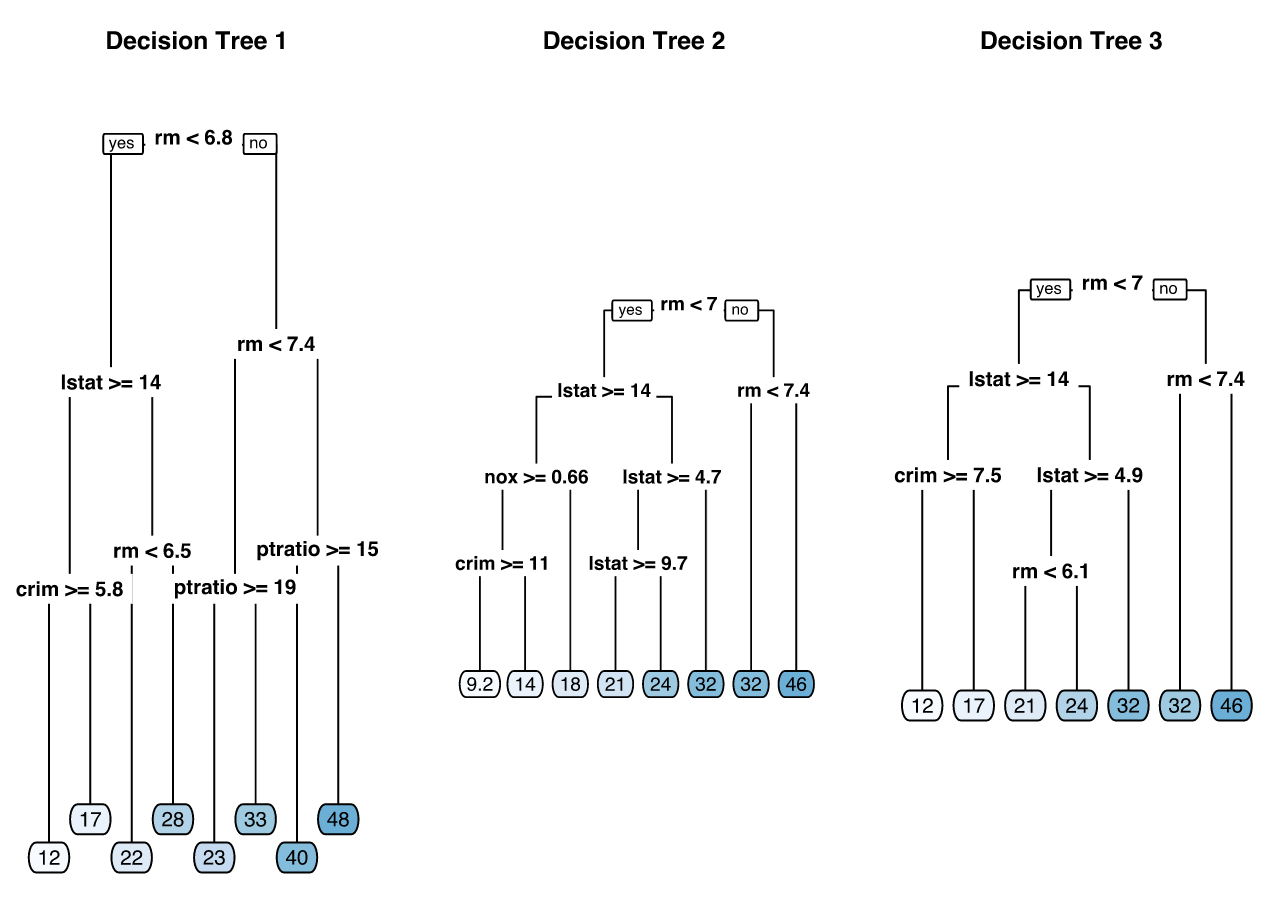
We create three decision trees based on three different samples of the data.
The first few partitions are fairly similar at the top of each tree; - they tend to differ closer to the terminal nodes.
These deeper nodes tend to overfit to specific attributes of the sample data;
Slightly different samples will result in highly variable estimate/ predicted values in the terminal nodes.
By pruning these lower level decision nodes, we can introduce a little bit of bias in our model that help to stabilize predictions and will tend to generalize better to new, unseen data.

Three decision trees based on three samples.

Cost complexity criterion

There is often a balance to be achieved in the depth and complexity of the tree to optimize predictive performance on some unseen data.
To find this balance, we grow a very large tree as showed and then prune it back to find an optimal subtree.
We find this subtree by using a cost complexity parameter ($\alpha$) that penalizes our objective function for the number of terminal nodes of the tree (T).

$\text{minimize}\{SSE + \alpha|T|\}$

The complexity value $\alpha$

For a given value of $\alpha$, we find the smallest pruned tree that has the lowest penalized error.
$\rightarrow$ A close association to the lasso $L_1$ norm penalty.
Smaller penalties tend to produce more complex models, which result in larger trees.
Larger penalties result in much smaller trees.
As a tree grows larger, the reduction in the SSE must be greater than the cost complexity penalty.
We evaluate multiple models across a spectrum of $\alpha$ and use cross-validation to identify the optimal $\alpha$ and the optimal subtree.

Fit a regression tree using `rpart`

The fitting process and the visual output of regression trees and classification trees are very similar.
Both use the formula method for expressing the model (similar to lm).
When fitting a regression tree, we need to set method = "anova".
By default, rpart will make an intelligent guess based on the data type of the response column
But it’s recommened to explictly set the method for reproducibility reasons (auto-guesser may change in future).

m1 <- rpart(formula = Sale_Price ~ .,data = ames_train,
            method  = "anova")

the `m1` output.

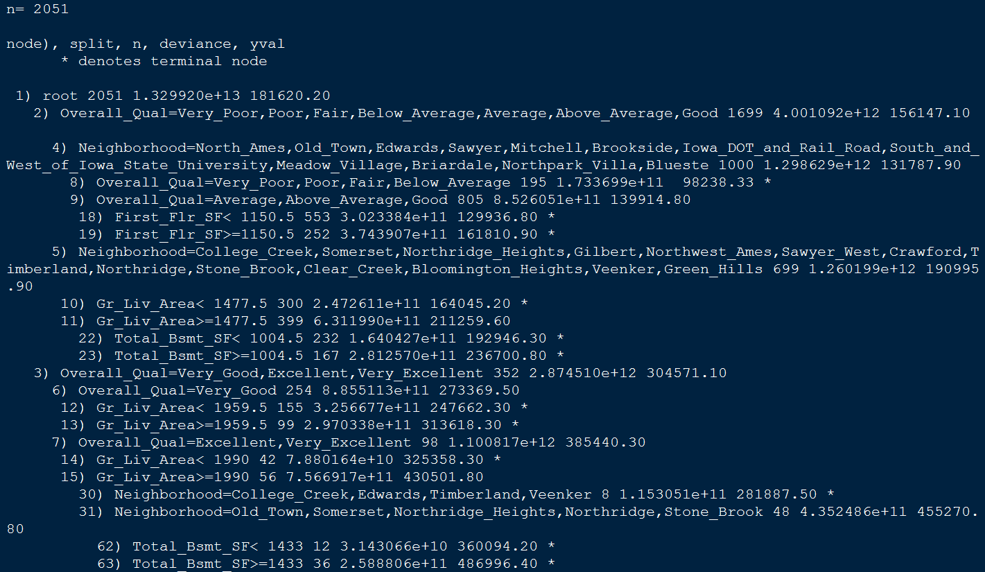
m1

## n= 2051 
## 
## node), split, n, deviance, yval
##       * denotes terminal node
## 
##  1) root 2051 1.273987e+13 180775.50  
##    2) Overall_Qual=Very_Poor,Poor,Fair,Below_Average,Average,Above_Average,Good 1703 4.032269e+12 156431.40  
##      4) Neighborhood=North_Ames,Old_Town,Edwards,Sawyer,Mitchell,Brookside,Iowa_DOT_and_Rail_Road,South_and_West_of_Iowa_State_University,Meadow_Village,Briardale,Northpark_Villa,Blueste 1015 1.360332e+12 131803.50  
##        8) First_Flr_SF< 1048.5 611 4.924281e+11 118301.50  
##         16) Overall_Qual=Very_Poor,Poor,Fair,Below_Average 152 1.053743e+11  91652.57 *
##         17) Overall_Qual=Average,Above_Average,Good 459 2.433622e+11 127126.40 *
##        9) First_Flr_SF>=1048.5 404 5.880574e+11 152223.50  
##         18) Gr_Liv_Area< 2007.5 359 2.957141e+11 145749.50 *
##         19) Gr_Liv_Area>=2007.5 45 1.572566e+11 203871.90 *
##      5) Neighborhood=College_Creek,Somerset,Northridge_Heights,Gilbert,Northwest_Ames,Sawyer_West,Crawford,Timberland,Northridge,Stone_Brook,Clear_Creek,Bloomington_Heights,Veenker,Green_Hills 688 1.148069e+12 192764.70  
##       10) Gr_Liv_Area< 1725.5 482 5.162415e+11 178531.00  
##         20) Total_Bsmt_SF< 1331 352 2.315412e+11 167759.00 *
##         21) Total_Bsmt_SF>=1331 130 1.332603e+11 207698.30 *
##       11) Gr_Liv_Area>=1725.5 206 3.056877e+11 226068.80 *
##    3) Overall_Qual=Very_Good,Excellent,Very_Excellent 348 2.759339e+12 299907.90  
##      6) Overall_Qual=Very_Good 249 9.159879e+11 268089.10  
##       12) Gr_Liv_Area< 1592.5 78 1.339905e+11 220448.90 *
##       13) Gr_Liv_Area>=1592.5 171 5.242201e+11 289819.70 *
##      7) Overall_Qual=Excellent,Very_Excellent 99 9.571896e+11 379937.20  
##       14) Gr_Liv_Area< 1947 42 7.265064e+10 325865.10 *
##       15) Gr_Liv_Area>=1947 57 6.712559e+11 419779.80  
##         30) Neighborhood=Old_Town,Edwards,Timberland 7 8.073100e+10 295300.00 *
##         31) Neighborhood=College_Creek,Somerset,Northridge_Heights,Northridge,Stone_Brook 50 4.668730e+11 437207.00  
##           62) Total_Bsmt_SF< 2168.5 40 1.923959e+11 408996.90 *
##           63) Total_Bsmt_SF>=2168.5 10 1.153154e+11 550047.30 *

Steps of the splits (m1) - explained

E.g., we start with 2051 observations at the root node (very beginning) and the first variable we split on (that optimizes a reduction in SSE) is Overall_Qual.
We see that at the first node all observations with

Overall_Qual=Very_Poor,Poor,Fair,Below_Average,Average,
Above_Average,Good

go to the 2nd branch.

The 3rd branch

The number of observations in this branch (1699), their average sales price (156147.10) and SSE (4.001092e+12) are listed.
In the 3rd branch we have 352 observations with

Overall_Qual=Very_Good,Excellent,Very_Excellent

their average sales prices is 304571.10 and the SEE in this region is 2.874510e+12. <!–
Overall_Qual is the most important variable that has the largest reduction in SEE initially
With those homes on the upper end of the quality spectrum having almost double the average sales price.

–>

Visualization with `rpart.plot`

In the default print it will show the percentage of data that fall to that node and the average sales price for that branch.
This tree contains 11 internal nodes resulting in 12 terminal nodes.
This tree is partitioning on 11 variables to produce its model.

The package `rpart.plot`

rpart.plot(m1)

Behind the scenes

There are 80 variables in ames_train. So what happened?

rpart is automatically applying a range of cost complexity $\alpha$ values to prune the tree.
To compare the error for each $\alpha$ value, rpart performs a 10-fold cross validation so that the error associated with a $\alpha$ value is computed on the hold-out validation data.

The `plotcp`

Lower x-axis - cost complexity - alpha

plotcp(m1)

The 1-SE rule - how many terminal nodes

Breiman et al. (1984) suggested to use the smallest tree within 1 standard deviation of the minimum cross validation error (aka the 1-SE rule).
Thus, we could use a tree with 9 terminal nodes and expect to get similar results within a small margin of error.
To illustrate the point of selecting a tree with 12 terminal nodes (or 9 if you go by the 1-SE rule), we can force rpart to generate a full tree by using cp = 0 (no penalty results in a fully grown tree).

Generate a full tree

After 12 terminal nodes, we see diminishing returns in error reduction as the tree grows deeper.
Thus, we can signifcantly prune our tree and still achieve minimal expected error.

m2 <- rpart(formula = Sale_Price ~ .,data=ames_train,
    method  = "anova",control = list(cp = 0, xval = 10))

control - a list of options that control details of the rpart algorithm.
cp - complexity parameter. Any split that does not decrease the overall lack of fit by a factor of cp is not attempted. For instance, with anova splitting, this means that the overall R-squared must increase by cp at each step (Pruning).
xval number of cross-validations.

Plot the result

plotcp(m2);abline(v = 12, lty = "dashed")

Automated tuning by default

rpart is performing some automated tuning by default, with an optimal subtree of 11 splits, 12 terminal nodes, and a cross-validated error of 0.272 (note that this error is equivalent to the predicted residual error sum of squares statistic (PRESS) but not the MSE).
We can perform additional tuning to try improve model performance.

The output `cptable`

m1$cptable

##            CP nsplit rel error    xerror       xstd
## 1  0.46690132      0 1.0000000 1.0009222 0.05855161
## 2  0.11961409      1 0.5330987 0.5347929 0.03116217
## 3  0.06955813      2 0.4134846 0.4151417 0.03058554
## 4  0.02559992      3 0.3439265 0.3461258 0.02207839
## 5  0.02196620      4 0.3183265 0.3242197 0.02182111
## 6  0.02023390      5 0.2963603 0.3074877 0.02129292
## 7  0.01674138      6 0.2761264 0.2963372 0.02106996
## 8  0.01188709      7 0.2593850 0.2795199 0.01903482
## 9  0.01127889      8 0.2474980 0.2762666 0.01936472
## 10 0.01109955      9 0.2362191 0.2699895 0.01902217
## 11 0.01060346     11 0.2140200 0.2672133 0.01883219
## 12 0.01000000     12 0.2034165 0.2635207 0.01881691

Tuning

In addition to the cost complexity ($\alpha$) parameter, it is also common to tune:

`minsplit`:

The minimum number of data points required to attempt a split before it is forced to create a terminal node. The default is 20. Making this smaller allows for terminal nodes that may contain only a handful of observations to create the predicted value.

`maxdepth`:

The maximum number of internal nodes between the root node and the terminal nodes. The default is 30, which is quite liberal and allows for fairly large trees to be built.

Special control argument

rpart uses a special control argument where we provide a list of hyperparameter values.
E.g., if we want a model with minsplit = 10 and maxdepth = 12, we could execute the following:

m3 <- rpart(formula = Sale_Price ~ .,data = ames_train,
    method  = "anova", control = list(minsplit = 10, 
                          maxdepth = 12, xval = 10)
)

The output `cptable` of model 3

m3$cptable

##            CP nsplit rel error    xerror       xstd
## 1  0.46690132      0 1.0000000 1.0004448 0.05850012
## 2  0.11961409      1 0.5330987 0.5343156 0.03093134
## 3  0.06955813      2 0.4134846 0.4148699 0.03035832
## 4  0.02559992      3 0.3439265 0.3455539 0.02190359
## 5  0.02196620      4 0.3183265 0.3259151 0.02168056
## 6  0.02023390      5 0.2963603 0.3062045 0.02114604
## 7  0.01674138      6 0.2761264 0.3061135 0.02176061
## 8  0.01188709      7 0.2593850 0.2917534 0.02058535
## 9  0.01127889      8 0.2474980 0.2872380 0.02441006
## 10 0.01109955      9 0.2362191 0.2850234 0.02440721
## 11 0.01060346     11 0.2140200 0.2829790 0.02334151
## 12 0.01000000     12 0.2034165 0.2735069 0.02260957

Grid search

We can avoid it to manually assess multiple models, by performing a grid search to automatically search across a range of differently tuned models to identify the optimal hyerparameter setting.
To perform a grid search we first create our hyperparameter grid. <!–
Here, we search a range of minsplit from 5-20 and vary maxdepth from 8-15 (since our original model found an optimal depth of 12). –>

hyper_grid <- expand.grid(
  minsplit = seq(5, 20, 1),
  maxdepth = seq(8, 15, 1)
)

The result are 128 combinations - 128 different models.

head(hyper_grid)

##   minsplit maxdepth
## 1        5        8
## 2        6        8
## 3        7        8
## 4        8        8
## 5        9        8
## 6       10        8

nrow(hyper_grid)

## [1] 128

A loop to autimate modeling

We iterate through each minsplit and maxdepth combination.
We save each model into its own list item.

models <- list()
for (i in 1:nrow(hyper_grid)) {
  # get minsplit, maxdepth values at row i
  minsplit <- hyper_grid$minsplit[i]
  maxdepth <- hyper_grid$maxdepth[i]
  # train a model and store in the list
  models[[i]] <- rpart(formula=Sale_Price~.,data=ames_train,
    method="anova",control=list(minsplit=minsplit,
                                maxdepth=maxdepth)
    )
}

A function to extract the minimum error

We create functions to extract the minimum error associated with the optimal cost complexity $\alpha$ value for each model.

# function to get optimal cp
get_cp <- function(x) {
  min    <- which.min(x$cptable[, "xerror"])
  cp <- x$cptable[min, "CP"] 
}

# function to get minimum error
get_min_error <- function(x) {
  min    <- which.min(x$cptable[, "xerror"])
  xerror <- x$cptable[min, "xerror"] 
}

Apply the functions

hyper_grid %>%
  mutate(
    cp    = purrr::map_dbl(models, get_cp),
    error = purrr::map_dbl(models, get_min_error)
    ) %>%
  arrange(error) %>%
  top_n(-5, wt = error)

##   minsplit maxdepth         cp     error
## 1       16       12 0.01060346 0.2628987
## 2        6       11 0.01000000 0.2645615
## 3       11       11 0.01000000 0.2650862
## 4       10       10 0.01000000 0.2655860
## 5        7       15 0.01000000 0.2656602

Exercise

Apply the final optimal model

Predict on our test dataset

The final optimal model

Apply the final optimal model:

optimal_tree <- rpart(formula = Sale_Price ~ .,
    data    = ames_train,method  = "anova",
    control = list(minsplit = 5, maxdepth = 13, cp = 0.0108982)
    )

Predict on our test dataset:

pred <- predict(optimal_tree, newdata = ames_test)

The final RMSE is 39145.39 which suggests that, on average, our predicted sales prices are about 39,145 Dollar off from the actual sales price.

RMSE(pred = pred, obs = ames_test$Sale_Price)

## [1] 39558.22

Exercise: `rpart` Kyphosis

Consider the Kyphosis data frame

1) Which variables are in the kyphosis dataset 2) Build a tree to classify Kyphosis from Age, Number and Start.

Consider the tree build above.

3) Which variables are used to explain Kyphosis presence? 4) How many observations contain the terminal nodes.

Consider the Kyphosis data frame.

5) Build a tree using the first 60 observations of kyphosis. 6) Predict the kyphosis presence for the other 21 observations. 7) Which is the misclassification rate (prediction error)

Exercise: `rpart` `iris`

Consider the `iris` data frame

1) Build a tree to classify Species from the other variables. 2) Plot the trees, add nodes information.

Consider the tree build before

3) Prune the the using median complexity parameter (cp) associated to the tree. 4) Plot in the same window, the pruned and the original tree. 5) In which terminal nodes is clasified each oobservations of iris? 6) Which Specie has a flower of Petal.Length greater than 2.45 and Petal.Width less than 1.75.

Advantages of regression trees

They are very interpretable.
Making predictions is fast (no complicated calculations, just looking up constants in the tree).
It’s easy to understand what variables are important for the prediction.
The internal nodes (splits) are those variables that most largely reduced the SSE.
If some data is missing, we might not be able to go all the way down the tree to a leaf, but we can still make a prediction by averaging all the leaves in the sub-tree.
The model provides a non-linear response, so it can work when the true regression surface is not smooth.
If it is smooth, the piecewise-constant surface can approximate it arbitrarily closely (with enough leaves).
There are fast, reliable algorithms to learn these trees.

Weaknesses of regression trees

Single regression trees have high variance, resulting in unstable predictions (an alternative subsample of training data can significantly change the terminal nodes).
Due to the high variance single regression trees have poor predictive accuracy.

Ensembling

Ensembles are machine learning methods for combining predictions from multiple separate models.

Bagging

attempts to reduce the chance of overfitting complex models.

It trains a large number of “strong” learners in parallel.
A strong learner is a model that’s relatively unconstrained.
Bagging then combines all the strong learners together in order to “smooth out” their predictions.

Boosting

attempts to improve the predictive flexibility of simple models.

It trains a large number of “weak” learners in sequence.
A weak learner is a constrained model (limit for max depth of tree).
Each one in the sequence focuses on learning from the mistakes of the one before it.
Boosting combines all the weak learners into a single strong learner.

Bagging and boosting

While bagging and boosting are both ensemble methods, they approach the problem from opposite directions.

Bagging uses complex base models and tries to “smooth out” their predictions, while boosting uses simple base models and tries to “boost” their aggregate complexity.

Bagging

Single tree models suffer from high variance, they are highly unstable and poor predictors.
Pruning helps, but there are alternative methods that exploite the variability of single trees in a way that can significantly improve performance.
Bootstrap aggregating (bagging) is one such approach (originally proposed by Breiman, 1996).
Bagging is a method for combining predictions from different regression or classification models.
The results of the models are then averaged - in the simplest case model predictions are included with the same weight.
The weights could depend on the quality of the model prediction, i.e. “good” models are more important than “bad” models.
Bagging leads to significantly improved predictions in the case of unstable models.

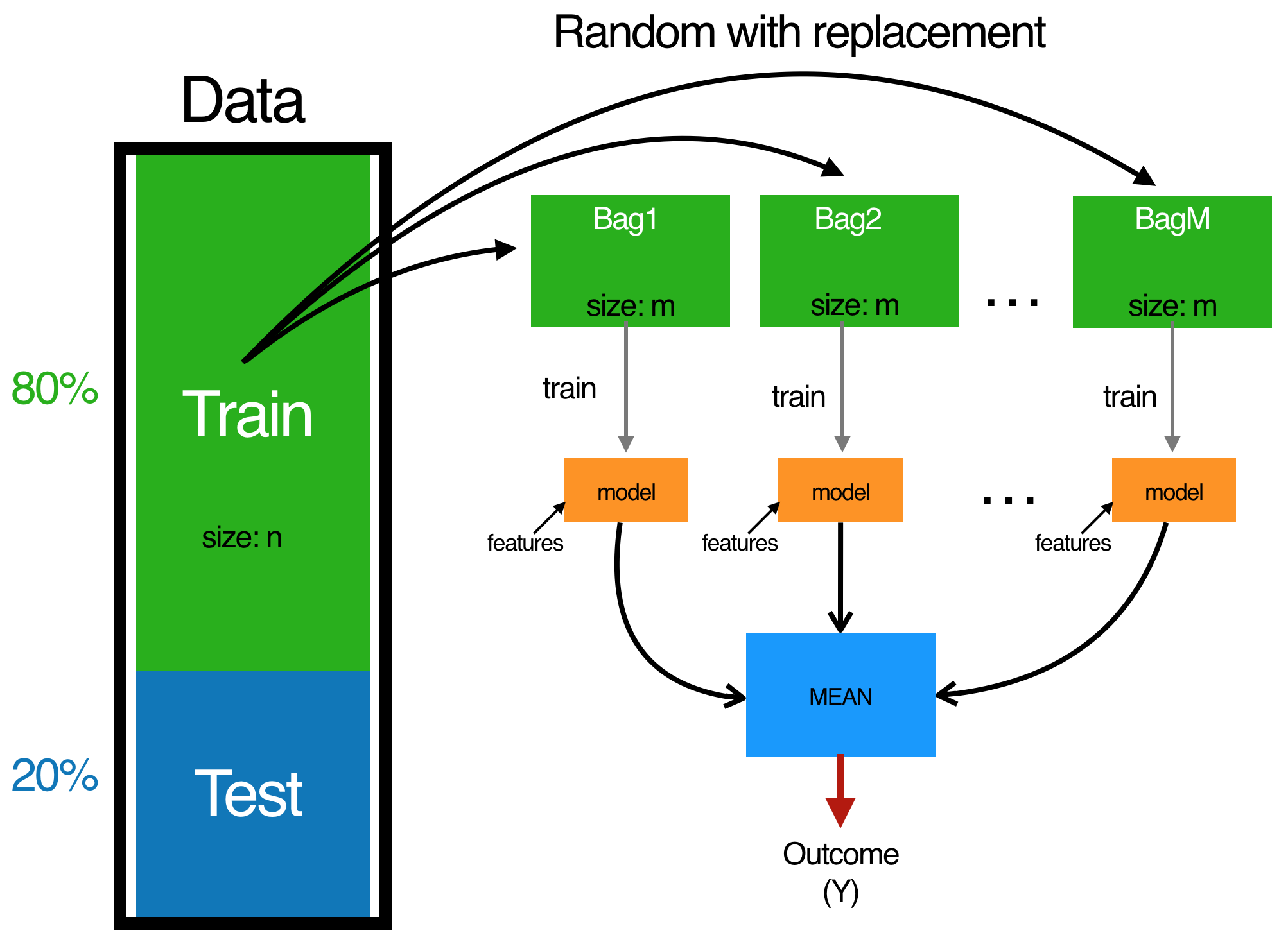
Bagging follows three simple steps:

1.) Create $m$ bootstrap samples from the training data. Bootstrapped samples allow us to create many slightly different data sets but with the same distribution as the overall training set.
2.) For each bootstrap sample train a single, unpruned regression tree.
3.) Average individual predictions from each tree to create an overall average predicted value.

The bagging process.

{ height=70% }

About bagging

This process can be applied to any regression or classification model;
It provides the greatest improvement for models that have high variance.
More stable parametric models such as linear regression and multi-adaptive regression splines tend to experience less improvement in predictive performance.
On average, a bootstrap sample will contain 63 per cent of the training data.
This leaves about 33 per cent ($\dfrac{1}{3}$) of the data out of the bootstrapped sample. We call this the out-of-bag (OOB) sample.
We can use the OOB observations to estimate the model’s accuracy, creating a natural cross-validation process.

Bagging with `ipred`

Fitting a bagged tree model is quite simple.
Instead of using rpart we use ipred::bagging.
We use coob = TRUE to use the OOB sample to estimate the test error.

Train bagged model

set.seed(123)
(bagged_m1 <- bagging(formula = Sale_Price ~ .,
  data    = ames_train,coob= TRUE))

## 
## Bagging regression trees with 25 bootstrap replications 
## 
## Call: bagging.data.frame(formula = Sale_Price ~ ., data = ames_train, 
##     coob = TRUE)
## 
## Out-of-bag estimate of root mean squared error:  36991.67

We see that our initial estimate error is close to 3000 Dollar less than the test error we achieved with our single optimal tree (36543 vs. 39145)

Things to note typically

The more trees the better - we are averaging over more high variance single trees.
We see a dramatic reduction in variance (and hence our error) and eventually the reduction in error will flatline <!–
signaling an appropriate number of trees to create a stable model. –>
You need less than 50 trees to stabilize the error.

Number of bootstrap samples

By default bagging performs 25 bootstrap samples and trees but we may require more. <!–
We can assess the error versus number of trees as below. –>

# assess 10-50 bagged trees
ntree <- 10:50 
# create empty vector to store OOB RMSE values
rmse <- vector(mode = "numeric", length = length(ntree))
for (i in seq_along(ntree)) {
  # reproducibility
  set.seed(123)   
  # perform bagged model
  model <- bagging(formula = Sale_Price ~ .,
  data=ames_train,coob= TRUE,nbagg=ntree[i]
)
  # get OOB error
  rmse[i] <- model$err   
}

Plot the result

The error is stabilizing at about 25 trees - we will improve by bagging more trees.

plot(ntree, rmse, type = 'l', lwd = 2)
abline(v = 25, col = "red", lty = "dashed")

Bagging with `caret`

Bagging with ipred is simple but there are some additional benefits of bagging with caret.

1.) Its easier to perform cross-validation. Although we can use the OOB error, performing cross validation will provide a more robust understanding of the true expected test error.

2.) We can assess variable importance across the bagged trees.

Excursus: Variable importance (vi)

vi measures help understand the results obtained from complex machine learning models
There is no general consensus on the “best” way to compute - or even define - the concept of variable importance.
See a list of many possible approaches to compute vi in the help file of the command varImp

?caret::varImp

vi refers to how much a given model “uses” that variable to make accurate predictions. The more a model relies on a variable to make predictions, the more important it is for the model.

A 10-fold cross-validated model.

# Specify 10-fold cross validation
ctrl <- trainControl(method = "cv",  number = 10) 

bagged_cv <- train(Sale_Price ~ .,data = ames_train,
  method = "treebag",trControl = ctrl,importance = TRUE)

treebag- means we use a bagging tree

Assess results

bagged_cv

## Bagged CART 
## 
## 2051 samples
##   80 predictor
## 
## No pre-processing
## Resampling: Cross-Validated (10 fold) 
## Summary of sample sizes: 1846, 1845, 1846, 1845, 1847, 1847, ... 
## Resampling results:
## 
##   RMSE      Rsquared   MAE     
##   35854.02  0.8009063  23785.85

Assess results with a plot (top 20 variables)

Here, variable importance is measured by assessing the total amount SSE is decreased by splits over a given predictor, averaged over all $m$ trees.

plot(varImp(bagged_cv), 20) 

Extensions

If we compare this to the test set out of sample we see that our cross-validated error estimate was very close.

pred <- predict(bagged_cv, ames_test)
RMSE(pred, ames_test$Sale_Price)

## [1] 35357.89

We have successfully reduced our error to about $35k;
Extensions of this bagging concept (random forests and GBMs) can significantly reduce this further.

Decision Trees

Regression tree vs. classification tree

library(rpart)

Grow a tree

fit <- rpart(Kyphosis ~ Age + Number + Start,
   method="class", data=kyphosis)

printcp(fit) # display the results

## 
## Classification tree:
## rpart(formula = Kyphosis ~ Age + Number + Start, data = kyphosis, 
##     method = "class")
## 
## Variables actually used in tree construction:
## [1] Age   Start
## 
## Root node error: 17/81 = 0.20988
## 
## n= 81 
## 
##         CP nsplit rel error xerror    xstd
## 1 0.176471      0   1.00000 1.0000 0.21559
## 2 0.019608      1   0.82353 1.1176 0.22433
## 3 0.010000      4   0.76471 1.1176 0.22433

plotcp(fit) # visualize cross-validation results

summary(fit) # detailed summary of splits

## Call:
## rpart(formula = Kyphosis ~ Age + Number + Start, data = kyphosis, 
##     method = "class")
##   n= 81 
## 
##           CP nsplit rel error   xerror      xstd
## 1 0.17647059      0 1.0000000 1.000000 0.2155872
## 2 0.01960784      1 0.8235294 1.117647 0.2243268
## 3 0.01000000      4 0.7647059 1.117647 0.2243268
## 
## Variable importance
##  Start    Age Number 
##     64     24     12 
## 
## Node number 1: 81 observations,    complexity param=0.1764706
##   predicted class=absent   expected loss=0.2098765  P(node) =1
##     class counts:    64    17
##    probabilities: 0.790 0.210 
##   left son=2 (62 obs) right son=3 (19 obs)
##   Primary splits:
##       Start  < 8.5  to the right, improve=6.762330, (0 missing)
##       Number < 5.5  to the left,  improve=2.866795, (0 missing)
##       Age    < 39.5 to the left,  improve=2.250212, (0 missing)
##   Surrogate splits:
##       Number < 6.5  to the left,  agree=0.802, adj=0.158, (0 split)
## 
## Node number 2: 62 observations,    complexity param=0.01960784
##   predicted class=absent   expected loss=0.09677419  P(node) =0.7654321
##     class counts:    56     6
##    probabilities: 0.903 0.097 
##   left son=4 (29 obs) right son=5 (33 obs)
##   Primary splits:
##       Start  < 14.5 to the right, improve=1.0205280, (0 missing)
##       Age    < 55   to the left,  improve=0.6848635, (0 missing)
##       Number < 4.5  to the left,  improve=0.2975332, (0 missing)
##   Surrogate splits:
##       Number < 3.5  to the left,  agree=0.645, adj=0.241, (0 split)
##       Age    < 16   to the left,  agree=0.597, adj=0.138, (0 split)
## 
## Node number 3: 19 observations
##   predicted class=present  expected loss=0.4210526  P(node) =0.2345679
##     class counts:     8    11
##    probabilities: 0.421 0.579 
## 
## Node number 4: 29 observations
##   predicted class=absent   expected loss=0  P(node) =0.3580247
##     class counts:    29     0
##    probabilities: 1.000 0.000 
## 
## Node number 5: 33 observations,    complexity param=0.01960784
##   predicted class=absent   expected loss=0.1818182  P(node) =0.4074074
##     class counts:    27     6
##    probabilities: 0.818 0.182 
##   left son=10 (12 obs) right son=11 (21 obs)
##   Primary splits:
##       Age    < 55   to the left,  improve=1.2467530, (0 missing)
##       Start  < 12.5 to the right, improve=0.2887701, (0 missing)
##       Number < 3.5  to the right, improve=0.1753247, (0 missing)
##   Surrogate splits:
##       Start  < 9.5  to the left,  agree=0.758, adj=0.333, (0 split)
##       Number < 5.5  to the right, agree=0.697, adj=0.167, (0 split)
## 
## Node number 10: 12 observations
##   predicted class=absent   expected loss=0  P(node) =0.1481481
##     class counts:    12     0
##    probabilities: 1.000 0.000 
## 
## Node number 11: 21 observations,    complexity param=0.01960784
##   predicted class=absent   expected loss=0.2857143  P(node) =0.2592593
##     class counts:    15     6
##    probabilities: 0.714 0.286 
##   left son=22 (14 obs) right son=23 (7 obs)
##   Primary splits:
##       Age    < 111  to the right, improve=1.71428600, (0 missing)
##       Start  < 12.5 to the right, improve=0.79365080, (0 missing)
##       Number < 3.5  to the right, improve=0.07142857, (0 missing)
## 
## Node number 22: 14 observations
##   predicted class=absent   expected loss=0.1428571  P(node) =0.1728395
##     class counts:    12     2
##    probabilities: 0.857 0.143 
## 
## Node number 23: 7 observations
##   predicted class=present  expected loss=0.4285714  P(node) =0.08641975
##     class counts:     3     4
##    probabilities: 0.429 0.571

# plot tree
plot(fit, uniform=TRUE,
   main="Classification Tree for Kyphosis")
text(fit, use.n=TRUE, all=TRUE, cex=.8)

Decision Trees and Random Forest

–>

Resources and links

Breimann (1984) - Classification and Regression Trees
Vignette for package partykit
Conditional Inference Trees
Conditional inference trees vs traditional decision trees
Video on tree based methods
An example of practical machine learning using R

Tree-Based Models

But:

The Idea

Explanation: decision tree

Example decission trees

Example

Model foundations

How to grow a regression tree - deciding on splits

How are these partions made?

The best split

Regression Trees - preparation

The Ames Housing data

Pruning

Three decision trees based on three samples.

Cost complexity criterion

The complexity value $\alpha$

Fit a regression tree using rpart

the m1 output.

Steps of the splits (m1) - explained

The 3rd branch

Visualization with rpart.plot

The package rpart.plot

Behind the scenes

The plotcp

The 1-SE rule - how many terminal nodes

Generate a full tree

Plot the result

Automated tuning by default

The output cptable

Tuning

minsplit:

maxdepth:

Special control argument

The output cptable of model 3

Grid search

A loop to autimate modeling

A function to extract the minimum error

Apply the functions

Exercise

Apply the final optimal model

Predict on our test dataset

The final optimal model

Apply the final optimal model:

Predict on our test dataset:

Exercise: rpart Kyphosis

Consider the Kyphosis data frame

Consider the tree build above.

Consider the Kyphosis data frame.

Exercise: rpart iris

Consider the iris data frame

Consider the tree build before

Advantages of regression trees

Weaknesses of regression trees

Ensembling

Bagging

Boosting

Bagging and boosting

Bagging

Bagging follows three simple steps:

The bagging process.

About bagging

Bagging with ipred

Train bagged model

Things to note typically

Number of bootstrap samples

Plot the result

Bagging with caret

Excursus: Variable importance (vi)

A 10-fold cross-validated model.

Assess results

Assess results with a plot (top 20 variables)

Extensions

Decision Trees

Resources and links

Fit a regression tree using `rpart`

the `m1` output.

Visualization with `rpart.plot`

The package `rpart.plot`

The `plotcp`

The output `cptable`

`minsplit`:

`maxdepth`:

The output `cptable` of model 3

Exercise: `rpart` Kyphosis

Exercise: `rpart` `iris`

Consider the `iris` data frame

Bagging with `ipred`

Bagging with `caret`