Machine Learning: Regularization methods

Insufficient Solution

When the number of features exceed the number of observations ($p>n$), the OLS solution matrix is not invertible.
This causes significant issues because it means:

(1) The least-squares estimates are not unique. There are an infinite set of solutions available and most of these solutions overfit the data.

(2) In many instances the result will be computationally infeasible.

To resolve this issue we can remove variables until $p<n$ and then fit an OLS regression model.
Although we can use pre-processing tools to apply this manual approach (Kuhn and Johnson, 2013, pp. 43-47), it can be cumbersome and prone to errors.

Regularized Regression

When we experience these concerns, one alternative is to use regularized regression (also commonly referred to as penalized models or shrinkage methods) to control the parameter estimates.
Regularized regression puts contraints on the magnitude of the coefficients and will progressively shrink them towards zero. This constraint helps to reduce the magnitude and fluctuations of the coefficients and will reduce the variance of our model.

Regularization

elitedatascience.com definition

Regularization is a technique used to prevent overfitting by artificially penalizing model coefficients.

It can discourage large coefficients (by dampening them).
It can also remove features entirely (by setting their coefficients to 0).
The “strength” of the penalty is tunable.

Wikipedia definition of Regularization

Regularization is the process of adding information in order to solve an ill-posed problem or to prevent overfitting.

Strenghts and weaknesses of regularization

Strengths:

Linear regression is straightforward to understand and explain, and can be regularized to avoid overfitting.
Linear models can be updated easily with new data

Weaknesses:

Linear regression in general performs poorly when there are non-linear relationships. - They are not naturally flexible enough to capture more complex patterns, and adding the right interaction terms or polynomials can be tricky and time-consuming.

Three regularized regression algorithms

{ height=40% }

Lasso regression

Absolute size of coefficients is penalized.
Coefficients can be exactly 0.

Ridge regression

Squared size of coefficients is penalized.
Smaller coefficients, but it doesn’t force them to 0.

Elastic-net

A mix of both absolute and squared size is penalzied. <!–
The ratio of the two penalty types should be tuned. –>

The objective function of regularized regression methods…

is very similar to OLS regression;
And a penalty parameter (P) is added.

$\text{minimize}\{SSE+P\}$

There are two main penalty parameters, which have a similar effect.
They constrain the size of the coefficients such that the only way the coefficients can increase is if we experience a comparable decrease in the sum of squared errors (SSE).

Preparations

Most of the following slides are based on the UC Business Analytics R Programming Guide

Necessary packages

library(rsample)  # data splitting 
library(glmnet)   # implementing regularized regression approaches
library(dplyr)    # basic data manipulation procedures
library(ggplot2)  # plotting
library(knitr)    # for tables

The example dataset

library(AmesHousing) 
ames_data <- AmesHousing::make_ames()

Create training (70%) and test (30%) sets

set.seed is used for reproducibility
initial_split is used to split data in training and test data

set.seed(123)
ames_split <- rsample::initial_split(ames_data, prop = .7, 
                            strata = "Sale_Price")
ames_train <- rsample::training(ames_split)
ames_test  <- rsample::testing(ames_split)

Ridge Regression

Ridge regression (Hoerl, 1970) controls the coefficients by adding $\lambda\sum_{j=1}^p\beta_j^2$ to the objective function.
This penalty parameter is referred to as “$L_2$” as it signifies a second-order penalty being used on the coefficients.

$\text{minimize}\{\text{SSE}+\lambda\sum_{j=1}^p\beta_j^2 \}$

This penalty parameter can take on a wide range of values, which is controlled by the tuning parameter $\lambda$.
When $\lambda=0$, there is no effect and our objective function equals the normal OLS regression objective function of simply minimizing SSE.
As $\lambda \rightarrow \infty$, the penalty becomes large and forces our coefficients to zero.

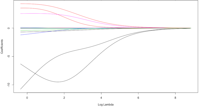
Exemplar coefficients

Exemplar coefficients have been regularized with $\lambda$ ranging from 0 to over 8,000 (log(8103)=9).

How to choose the right $\lambda$

Although these coefficients were scaled and centered prior to the analysis, you will notice that some are extremely large when $\lambda\rightarrow 0$.
We have a large negative parameter that fluctuates until $log(\lambda)\approx 2$ where it then continuously shrinks to zero.
This is indicates multicollinearity and likely illustrates that constraining our coefficients with $log(\lambda)>2$ may reduce the variance, and therefore the error, in our model.
But how do we find the amount of shrinkage (or $\lambda$) that minimizes our error?

Implementation in `glmnet`

plot(density(ames_data$Sale_Price),main="")

glmnet does not use the formula method (y ~ x) so prior to modeling we need to create our feature and target set.
The model.matrix function is used on our feature set, which will automatically dummy encode qualitative variables
We also log transform our response variable due to its skeweness.

Training and testing feature model matrices and response vectors.

We use model.matrix(...)[, -1] to discard the intercept

ames_train_x <- model.matrix(Sale_Price ~ ., ames_train)[, -1]
ames_train_y <- log(ames_train$Sale_Price)

ames_test_x <- model.matrix(Sale_Price ~ ., ames_test)[, -1]
ames_test_y <- log(ames_test$Sale_Price)

# What is the dimension of of your feature matrix?
dim(ames_train_x)

## [1] 2054  307

Behind the scenes

The alpha parameter tells glmnet to perform a Ridge ($\alpha = 0$), Lasso ($\alpha = 1$), or Elastic Net $(0\leq \alpha \leq 1)$ model.
Behind the scenes, glmnet is doing two things that you should be aware of:

(1.) It is essential that predictor variables are standardized when performing regularized regression. glmnet performs this for you. If you standardize your predictors prior to glmnet you can turn this argument off with standardize=FALSE.

(2.) glmnet will perform Ridge models across a wide range of $\lambda$ parameters, which are illustrated in the figure on the next slide.

ames_ridge <- glmnet(x = ames_train_x,y = ames_train_y,
  alpha = 0)

A wide range of $\lambda$ parameters

plot(ames_ridge, xvar = "lambda")

$\lambda$ values in `glmnet`

We can see the exact $\lambda$ values applied with ames_ridge$lambda.
You can specify your own $\lambda$ values,
By default glmnet applies 100 $\lambda$ values that are data derived.
Normally you will have little need to adjust the default $\lambda$ values.

head(ames_ridge$lambda)

## [1] 289.0010 263.3270 239.9337 218.6187 199.1972 181.5011

Access the coefficients with `coef`.

The coefficients are stored for each model in order of largest to smallest $\lambda$.
The coefficients for the Gr_Liv_Area and TotRms_AbvGrd features for the largest $\lambda$ (279.1035) and smallest $\lambda$ (0.02791035) are visible.
The largest $\lambda$ value has pushed these coefficients to nearly 0.

coef(ames_ridge)[c("Gr_Liv_Area", "TotRms_AbvGrd"),100]

##   Gr_Liv_Area TotRms_AbvGrd 
##  0.0001108687  0.0083032186

coef(ames_ridge)[c("Gr_Liv_Area", "TotRms_AbvGrd"), 1] 

##   Gr_Liv_Area TotRms_AbvGrd 
##  5.848028e-40  1.341550e-37

But how much improvement we are experiencing in our model.

Tuning

Recall that $\lambda$ is a tuning parameter that helps to control our model from over-fitting to the training data.
To identify the optimal $\lambda$ value we need to perform cross-validation (CV).
cv.glmnet provides a built-in option to perform k-fold CV, and by default, performs 10-fold CV.

ames_ridge <- cv.glmnet(x = ames_train_x,y = ames_train_y,
  alpha = 0)

Results of cv Ridge regression

plot(ames_ridge)

The plot illustrates the 10-fold CV mean squared error (MSE) across the $\lambda$ values.
We see no substantial improvement;

The plot explained (I)

As we constrain our coefficients with $log(\lambda)\leq 0$ penalty, the MSE rises considerably.
The numbers at the top of the plot (301) just refer to the number of variables in the model.
Ridge regression does not force any variables to exactly zero so all features will remain in the model.

The plot explained (II)

min(ames_ridge$cvm)       # minimum MSE

## [1] 0.01955871

ames_ridge$lambda.min     # lambda for this min MSE

## [1] 0.1542312

# 1 st.error of min MSE
ames_ridge$cvm[ames_ridge$lambda == ames_ridge$lambda.1se]  

## [1] 0.02160821

ames_ridge$lambda.1se  # lambda for this MSE

## [1] 0.5169216

The plot explained (III)

The advantage of identifying the $\lambda$ with an MSE within one standard error becomes more obvious with the Lasso and Elastic Net models.
For now we can assess this visually.
We plot the coefficients across the $\lambda$ values and the dashed red line represents the largest $\lambda$ that falls within one standard error of the minimum MSE.
This shows you how much we can constrain the coefficients while still maximizing predictive accuracy.

ames_ridge_min <- glmnet(x = ames_train_x,y = ames_train_y,
  alpha = 0)

Coefficients across the $\lambda$ values

plot(ames_ridge_min, xvar = "lambda")
abline(v = log(ames_ridge$lambda.1se), col = "red", 
       lty = "dashed")

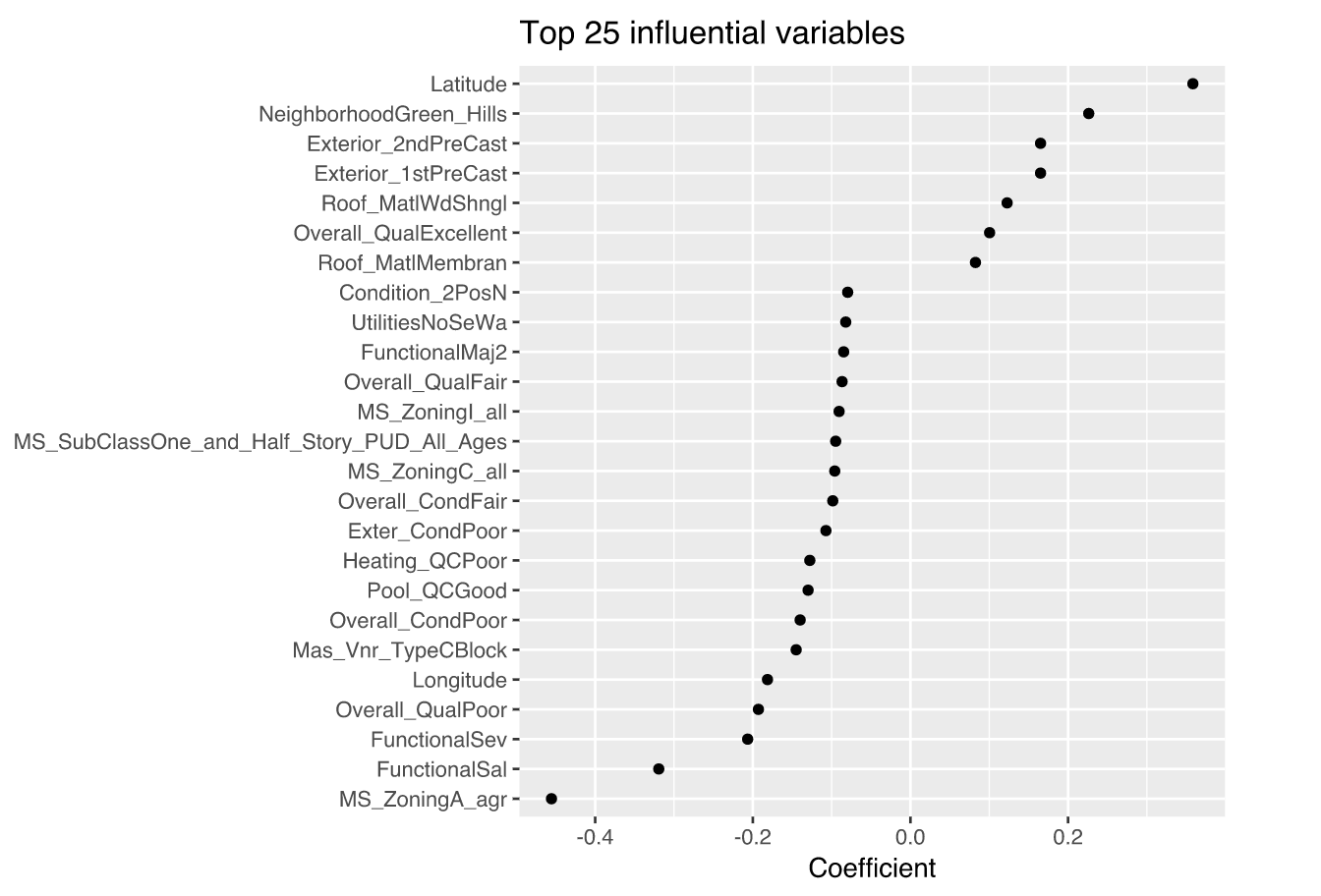
Advantages and Disadvantages

The Ridge regression model has pushed many of the correlated features towards each other rather than allowing for one to be wildly positive and the other wildly negative.
Many of the non-important features have been pushed closer to zero.
We have reduced the noise in our data $\Rightarrow$ more clarity in identifying the true signals.

coef(ames_ridge, s = "lambda.1se") %>%
  filter(row != "(Intercept)") %>%
  top_n(25, wt = abs(value)) %>%
  ggplot(aes(value, reorder(row, value))) +
  geom_point() +
  ggtitle("Top 25 influential variables") +
  xlab("Coefficient") +
  ylab(NULL)

Top 25 influential variables

Exercise: ridge regression (I)

1) Load the lars package and the diabetes dataset 2) Load the glmnet package to implement ridge regression.

The dataset has three matrices x, x2 and y. x has a smaller set of independent variables while x2 contains the full set with quadratic and interaction terms. y is the dependent variable which is a quantitative measure of the progression of diabetes.

3) Generate separate scatterplots with the line of best fit for all the predictors in x with y on the vertical axis.

4) Regress y on the predictors in x using OLS. We will use this result as benchmark for comparison.

Exercise: ridge regression (II)

5) Fit the ridge regression model using the glmnet function and plot the trace of the estimated coefficients against lambdas. Note that coefficients are shrunk closer to zero for higher values of lambda.

6) Use the cv.glmnet function to get the cross validation curve and the value of lambda that minimizes the mean cross validation error.

7) Using the minimum value of lambda from the previous exercise, get the estimated beta matrix. Note that coefficients are lower than least squares estimates.

8) To get a more parsimonious model we can use a higher value of lambda that is within one standard error of the minimum. Use this value of lambda to get the beta coefficients. Note the shrinkage effect on the estimates.

Exercise: ridge regression (III)

9) Split the data randomly between a training set (80%) and test set (20%). We will use these to get the prediction standard error for least squares and ridge regression models.

10) Fit the ridge regression model on the training and get the estimated beta coefficients for both the minimum lambda and the higher lambda within 1-standard error of the minimum.

11) Get predictions from the ridge regression model for the test set and calculate the prediction standard error. Do this for both the minimum lambda and the higher lambda within 1-standard error of the minimum.

12) Fit the least squares model on the training set.

13) Get predictions from the least squares model for the test set and calculate the prediction standard error.

Ridge and Lasso

A Ridge model…

… is good if we need to retain all features, yet reduce the noise that less influential variables may create and minimize multicollinearity.
… does not perform feature selection. If greater interpretation is necessary where you need to reduce the signal in your data to a smaller subset then a Lasso model may be preferable.

We could remove less important variables.
We can do that manually by examining p-values of coefficients and discarding those variables whose coefficients are not significant.
But this can become tedious for classification problems with many independent variables

Lasso Regression

Originally introduced in geophysics literature in 1986
The least absolute shrinkage and selection operator (Lasso) model was rediscovered and popularized in 1996 by Robert Tibshirani
It is an alternative to Ridge regression that has a small modification to the penalty in the objective function.
Rather than the $L_2$ penalty we use the following $L_1$ penalty $\lambda\sum_{j=1}^p \beta_j $ in the objective function.

$\text{minimize} \{\text{SSE}+\lambda\sum_{j=1}^p |\beta_j|\}$

Lasso penalty pushes coefficients to zero

$Lasso regression coefficients as $\lambda$ grows from $0 \rightarrow \infty$.$ { heigth=60% }

Lasso improves the model with regularization and conducts automated feature selection.

The reduction of coefficients

15 variables for $\text{log}(\lambda)=-5$
12 variables for $\text{log}(\lambda)=-1$
3 variables for $\text{log}(\lambda)=1$

When a data set has many features, Lasso can be used to identify and extract those features with the largest (and most consistent) signal.

Implementation Lasso regression to ames data

Implementing Lasso follows the same logic as implementing the Ridge model, we just need to switch $\alpha = 1$ within glmnet.

ames_lasso<-glmnet(x=ames_train_x,y=ames_train_y,alpha=1)

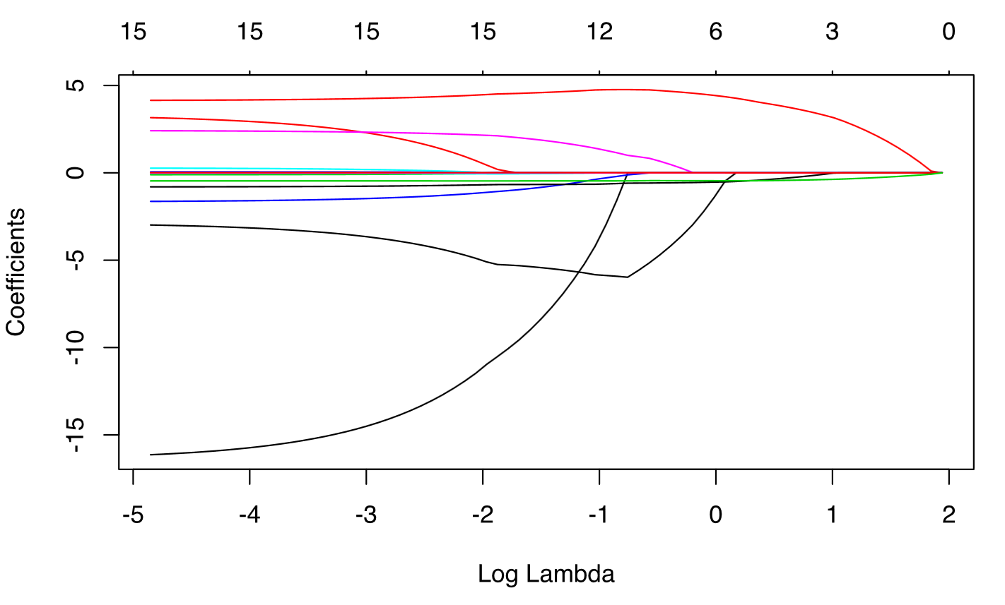
A quick drop in number of features

Very large coefficients for ols (highly correlated)
As model is constrained - these noisy features are pushed to 0.
CV is necessary to determine right value for $\lambda$

plot(ames_lasso, xvar = "lambda")

Tuning with `cv.glmnet`

cv.glmnet with alpha=1 is used to perform cv.

ames_lasso<-cv.glmnet(x=ames_train_x,y=ames_train_y,alpha=1)
names(ames_lasso)

##  [1] "lambda"     "cvm"        "cvsd"       "cvup"       "cvlo"      
##  [6] "nzero"      "name"       "glmnet.fit" "lambda.min" "lambda.1se"

MSE for cross validation

MSE can be minimized with $-6\leq log (\lambda) \leq -4$
Also the number of features can be reduced ($156 \leq p \leq 58$)

plot(ames_lasso)

Minimum and one standard error MSE and $\lambda$ values.

min(ames_lasso$cvm) # minimum MSE

## [1] 0.02246344

ames_lasso$lambda.min # lambda for this min MSE

## [1] 0.00332281

# 1 st.error of min MSE
ames_lasso$cvm[ames_lasso$lambda == ames_lasso$lambda.1se]  

## [1] 0.02482119

ames_lasso$lambda.1se  # lambda for this MSE

## [1] 0.01472211

MSE within one standard error

The advantage of identifying the $\lambda$ with an MSE within one standard error becomes more obvious.
If we use the $\lambda$ that drives the minimum MSE we can reduce our feature set from 307 down to less than 160.
There is some variability with this MSE and we can assume that we can achieve a similar MSE with a slightly more constrained model (only 63 features).
If describing and interpreting the predictors is an important outcome of your analysis, this will help.

Model with minimum MSE

plot(ames_lasso, xvar = "lambda")
abline(v=log(ames_lasso$lambda.min),col="red",lty="dashed")
abline(v=log(ames_lasso$lambda.1se),col="red",lty="dashed")

Lasso for other models than least squares

Though originally defined for least squares, Lasso regularization is easily extended to a wide variety of statistical models including generalized linear models, generalized estimating equations, proportional hazards models, and M-estimators, in a straightforward fashion.
Lasso’s ability to perform subset selection relies on the form of the constraint and has a variety of interpretations including in terms of geometry, Bayesian statistics, and convex analysis.
The Lasso is closely related to basis pursuit denoising.

Advantages and Disadvantages

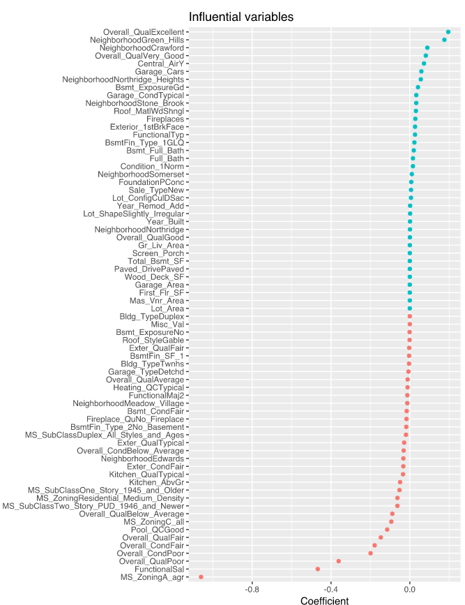
Similar to Ridge, the Lasso pushes many of the collinear features towards each other rather than allowing for one to be wildly positive and the other wildly negative.
Unlike Ridge, the Lasso will actually push coefficients to zero and perform feature selection.
This simplifies and automates the process of identifying those feature most influential to predictive accuracy.

Rcode for plotting influential variables

coef(ames_lasso, s = "lambda.1se") %>%
  tidy() %>%
  filter(row != "(Intercept)") %>%
  ggplot(aes(value, reorder(row, value), color = value > 0)) +
  geom_point(show.legend = FALSE) +
  ggtitle("Influential variables") +
  xlab("Coefficient") +
  ylab(NULL)

Plot Influential variables

MSE for Ridge and Lasso

# minimum Ridge MSE
min(ames_ridge$cvm)

## [1] 0.01955871

# minimum Lasso MSE
min(ames_lasso$cvm)

## [1] 0.02246344

Elastic net

Elastic-Net is a compromise between Lasso and Ridge.
Elastic-Net penalizes a mix of both absolute and squared size.
- The ratio of the two penalty types should be tuned.
- The overall strength should also be tuned.

Elastic Nets

A generalization of the Ridge and Lasso models is the Elastic Net (Zou and Hastie, 2005), which combines the two penalties.

$minimize \{SSE+\lambda \sum^p_{j=1} \beta^2_j+\lambda_2\sum_{j=1}^p |\beta_j|\}$

Summary overview

A result of Lasso is that typically when two strongly correlated features are pushed towards zero, one may be pushed fully to zero while the other remains in the model.
The process of one being in and one being out is not very systematic.
In contrast, the Ridge regression penalty is a little more effective in systematically reducing correlated features together.
The advantage of the Elastic Net model is that it enables effective regularization via the Ridge penalty with the feature selection characteristics of the Lasso penalty.

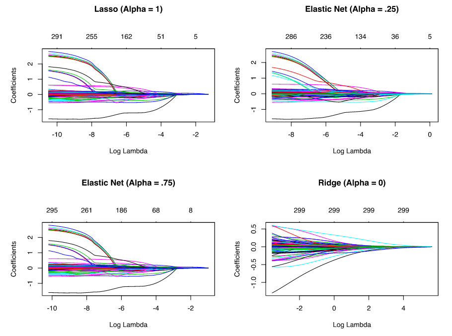
Implementation

alpha=.5 performs an equal combination of penalties

lasso    <- glmnet(ames_train_x, ames_train_y, alpha = 1.0) 
elastic1 <- glmnet(ames_train_x, ames_train_y, alpha = 0.25) 
elastic2 <- glmnet(ames_train_x, ames_train_y, alpha = 0.75) 
ridge    <- glmnet(ames_train_x, ames_train_y, alpha = 0.0)

The four model results plottet

Tuning the Elastic Net model

$\lambda$ is the primary tuning parameter in Ridge and Lasso models.
With elastic nets, we want to tune the $\lambda$ and the $\alpha$ parameters.
To set up our tuning, we create a common fold_id, which just allows us to apply the same CV folds to each model.

# maintain the same folds across all models
fold_id <- sample(1:10, size = length(ames_train_y), 
                  replace=TRUE)

Creation of a tuning grid

We then create a tuning grid that searches across a range of alphas from 0-1, and empty columns where we’ll dump our model results into.

# search across a range of alphas
tuning_grid <- tibble::tibble(
  alpha      = seq(0, 1, by = .1),
  mse_min    = NA,
  mse_1se    = NA,
  lambda_min = NA,
  lambda_1se = NA
)

Iteration over $\alpha$ values - Elastic Net

Now we can iterate over each $\alpha$ value, apply a CV Elastic Net, and extract the minimum and one standard error MSE values and their respective $\lambda$ values.

for(i in seq_along(tuning_grid$alpha)) {
  # fit CV model for each alpha value
  fit <- cv.glmnet(ames_train_x, ames_train_y, 
                   alpha = tuning_grid$alpha[i], 
                   foldid = fold_id)
  # extract MSE and lambda values
tuning_grid$mse_min[i]<-fit$cvm[fit$lambda==fit$lambda.min]
tuning_grid$mse_1se[i]<-fit$cvm[fit$lambda==fit$lambda.1se]
tuning_grid$lambda_min[i]<-fit$lambda.min
tuning_grid$lambda_1se[i]<-fit$lambda.1se
}

The resulting tuning grid

tuning_grid

## # A tibble: 11 x 5
##    alpha mse_min mse_1se lambda_min lambda_1se
##    <dbl>   <dbl>   <dbl>      <dbl>      <dbl>
##  1   0    0.0198  0.0227    0.141       0.623 
##  2   0.1  0.0205  0.0237    0.0365      0.134 
##  3   0.2  0.0210  0.0243    0.0182      0.0736
##  4   0.3  0.0213  0.0249    0.0122      0.0539
##  5   0.4  0.0215  0.0249    0.00912     0.0404
##  6   0.5  0.0216  0.0250    0.00729     0.0323
##  7   0.6  0.0217  0.0255    0.00608     0.0296
##  8   0.7  0.0218  0.0255    0.00521     0.0253
##  9   0.8  0.0219  0.0255    0.00456     0.0222
## 10   0.9  0.0219  0.0255    0.00405     0.0197
## 11   1    0.0220  0.0256    0.00365     0.0177

Plot the MSE

If we plot the MSE $\pm$ one standard error for the optimal $\lambda$ value for each alpha setting, we see that they all fall within the same level of accuracy.
We could select a full Lasso model with $\lambda=0.02062776$, gain the benefits of its feature selection capability and reasonably assume no loss in accuracy.

tuning_grid %>%
  mutate(se = mse_1se - mse_min) %>%
  ggplot(aes(alpha, mse_min)) +
  geom_line(size = 2) +
  geom_ribbon(aes(ymax = mse_min + se, ymin = mse_min - se), 
              alpha = .25) +
  ggtitle("MSE +/- one standard error")

MSE +/- one standard error

Predicting

With the preferred model, you can predict the same model on a new data set.
The only caveat is you need to supply predict an s parameter with the preferred models $\lambda$ value.
E.g., here we create a Lasso model, with a minimum MSE of 0.022.

# some best model
cv_lasso   <- cv.glmnet(ames_train_x, ames_train_y, alpha = 1.0)
min(cv_lasso$cvm)

## [1] 0.02036225

I use the minimum $\lambda$ value to predict on the unseen test set and obtain a slightly lower MSE of 0.015.

# predict
pred <- predict(cv_lasso, s = cv_lasso$lambda.min, ames_test_x)
mean((ames_test_y - pred)^2)

## [1] 0.02040651

The package `caret` - Classification and Regression Training

Vignette for the `caret` package

library(caret)
train_control <- trainControl(method = "cv", number = 10)
caret_mod <- train(x = ames_train_x,y = ames_train_y,
                   method = "glmnet",
                   preProc = c("center", "scale", "zv", "nzv"),
                   trControl = train_control,
                   tuneLength = 10)

Output for `caret` model

caret_mod

## glmnet 
## 
## 2054 samples
##  307 predictor
## 
## Pre-processing: centered (113), scaled (113), remove (194) 
## Resampling: Cross-Validated (10 fold) 
## Summary of sample sizes: 1849, 1848, 1847, 1850, 1849, 1849, ... 
## Resampling results across tuning parameters:
## 
##   alpha  lambda        RMSE       Rsquared   MAE       
##   0.1    0.0001335259  0.1529759  0.8626587  0.09899496
##   0.1    0.0003084622  0.1529697  0.8626702  0.09899085
##   0.1    0.0007125878  0.1527312  0.8630945  0.09882473
##   0.1    0.0016461703  0.1523040  0.8638461  0.09858775
##   0.1    0.0038028670  0.1518043  0.8647353  0.09829651
##   0.1    0.0087851163  0.1511589  0.8658996  0.09792048
##   0.1    0.0202947586  0.1512482  0.8658861  0.09846301
##   0.1    0.0468835259  0.1542133  0.8616162  0.10095388
##   0.1    0.1083070283  0.1613716  0.8525304  0.10562397
##   0.1    0.2502032890  0.1783894  0.8378278  0.11798124
##   0.2    0.0001335259  0.1530144  0.8625906  0.09901019
##   0.2    0.0003084622  0.1529054  0.8627844  0.09893138
##   0.2    0.0007125878  0.1526093  0.8633042  0.09873037
##   0.2    0.0016461703  0.1520597  0.8642754  0.09843475
##   0.2    0.0038028670  0.1515362  0.8652246  0.09801179
##   0.2    0.0087851163  0.1511130  0.8660407  0.09800962
##   0.2    0.0202947586  0.1531822  0.8629272  0.10015289
##   0.2    0.0468835259  0.1583264  0.8557192  0.10357302
##   0.2    0.1083070283  0.1713989  0.8406963  0.11319420
##   0.2    0.2502032890  0.2015887  0.8196545  0.13607965
##   0.3    0.0001335259  0.1530175  0.8625852  0.09901246
##   0.3    0.0003084622  0.1528417  0.8628943  0.09887464
##   0.3    0.0007125878  0.1524303  0.8636143  0.09862411
##   0.3    0.0016461703  0.1519261  0.8645281  0.09829674
##   0.3    0.0038028670  0.1513782  0.8655399  0.09792851
##   0.3    0.0087851163  0.1517901  0.8649707  0.09874489
##   0.3    0.0202947586  0.1548532  0.8604377  0.10124984
##   0.3    0.0468835259  0.1631931  0.8487612  0.10712019
##   0.3    0.1083070283  0.1804627  0.8317568  0.12000176
##   0.3    0.2502032890  0.2242488  0.8048855  0.15383093
##   0.4    0.0001335259  0.1530032  0.8626107  0.09900104
##   0.4    0.0003084622  0.1527835  0.8629949  0.09883071
##   0.4    0.0007125878  0.1522777  0.8638796  0.09853749
##   0.4    0.0016461703  0.1517960  0.8647653  0.09816823
##   0.4    0.0038028670  0.1512813  0.8657246  0.09790412
##   0.4    0.0087851163  0.1527729  0.8634153  0.09973034
##   0.4    0.0202947586  0.1567219  0.8575524  0.10244652
##   0.4    0.0468835259  0.1674084  0.8431901  0.11030906
##   0.4    0.1083070283  0.1900641  0.8220999  0.12713979
##   0.4    0.2502032890  0.2456477  0.7968665  0.17219318
##   0.5    0.0001335259  0.1529694  0.8626695  0.09897170
##   0.5    0.0003084622  0.1527206  0.8631031  0.09877948
##   0.5    0.0007125878  0.1521743  0.8640690  0.09847427
##   0.5    0.0016461703  0.1517015  0.8649410  0.09808645
##   0.5    0.0038028670  0.1514410  0.8654740  0.09816784
##   0.5    0.0087851163  0.1535069  0.8622717  0.10039370
##   0.5    0.0202947586  0.1585892  0.8546972  0.10366586
##   0.5    0.0468835259  0.1711919  0.8386196  0.11310210
##   0.5    0.1083070283  0.1988715  0.8144491  0.13394394
##   0.5    0.2502032890  0.2677720  0.7874492  0.19208881
##   0.6    0.0001335259  0.1529457  0.8627110  0.09894655
##   0.6    0.0003084622  0.1526476  0.8632329  0.09872871
##   0.6    0.0007125878  0.1521007  0.8642136  0.09841560
##   0.6    0.0016461703  0.1516403  0.8650668  0.09805262
##   0.6    0.0038028670  0.1516698  0.8651021  0.09848230
##   0.6    0.0087851163  0.1541771  0.8612517  0.10084110
##   0.6    0.0202947586  0.1606510  0.8515691  0.10511838
##   0.6    0.0468835259  0.1751425  0.8337697  0.11597593
##   0.6    0.1083070283  0.2072075  0.8085757  0.14014121
##   0.6    0.2502032890  0.2895134  0.7807597  0.21111363
##   0.7    0.0001335259  0.1529182  0.8627588  0.09892152
##   0.7    0.0003084622  0.1525582  0.8633865  0.09868078
##   0.7    0.0007125878  0.1520463  0.8643179  0.09835732
##   0.7    0.0016461703  0.1515912  0.8651754  0.09802856
##   0.7    0.0038028670  0.1519555  0.8646544  0.09881899
##   0.7    0.0087851163  0.1548004  0.8603025  0.10119692
##   0.7    0.0202947586  0.1627999  0.8483414  0.10680467
##   0.7    0.0468835259  0.1792009  0.8286142  0.11899322
##   0.7    0.1083070283  0.2158269  0.8020943  0.14685245
##   0.7    0.2502032890  0.3123587  0.7639857  0.23129960
##   0.8    0.0001335259  0.1528934  0.8628024  0.09889940
##   0.8    0.0003084622  0.1524796  0.8635221  0.09864034
##   0.8    0.0007125878  0.1519877  0.8644285  0.09830023
##   0.8    0.0016461703  0.1515406  0.8652735  0.09802800
##   0.8    0.0038028670  0.1522942  0.8641256  0.09918411
##   0.8    0.0087851163  0.1554853  0.8592392  0.10161487
##   0.8    0.0202947586  0.1649098  0.8451450  0.10842937
##   0.8    0.0468835259  0.1832344  0.8233507  0.12199727
##   0.8    0.1083070283  0.2242570  0.7962765  0.15379654
##   0.8    0.2502032890  0.3360986  0.7248864  0.25185135
##   0.9    0.0001335259  0.1528683  0.8628464  0.09887948
##   0.9    0.0003084622  0.1524011  0.8636585  0.09859931
##   0.9    0.0007125878  0.1519283  0.8645367  0.09825245
##   0.9    0.0016461703  0.1514541  0.8654270  0.09800839
##   0.9    0.0038028670  0.1526743  0.8635214  0.09958496
##   0.9    0.0087851163  0.1562250  0.8580869  0.10208126
##   0.9    0.0202947586  0.1667279  0.8425633  0.10988380
##   0.9    0.0468835259  0.1869510  0.8187765  0.12486550
##   0.9    0.1083070283  0.2328192  0.7897299  0.16118585
##   0.9    0.2502032890  0.3598416  0.6471565  0.27230177
##   1.0    0.0001335259  0.1528421  0.8628890  0.09885896
##   1.0    0.0003084622  0.1523370  0.8637698  0.09856552
##   1.0    0.0007125878  0.1518838  0.8646164  0.09822006
##   1.0    0.0016461703  0.1514135  0.8655058  0.09802221
##   1.0    0.0038028670  0.1530411  0.8629353  0.09994305
##   1.0    0.0087851163  0.1570340  0.8568153  0.10261590
##   1.0    0.0202947586  0.1683894  0.8402729  0.11115096
##   1.0    0.0468835259  0.1904441  0.8148559  0.12743546
##   1.0    0.1083070283  0.2409139  0.7855310  0.16832017
##   1.0    0.2502032890  0.3805446  0.5646772  0.29026265
## 
## RMSE was used to select the optimal model using the smallest value.
## The final values used for the model were alpha = 0.2 and lambda
##  = 0.008785116.

Which regularization method should we choose?

There’s no “best” type of penalty. It depends on the dataset and the problem.
We recommend trying different algorithms that use a range of penalty strengths as part of the tuning process

Advantages and Disadvantages

The advantage of the Elastic Net model is that it enables effective regularization via the Ridge penalty with the feature selection characteristics of the Lasso penalty.
Elastic Nets allow us to control multicollinearity concerns, perform regression when $p>n$, and reduce excessive noise in our data so that we can isolate the most influential variables while balancing prediction accuracy.
Elastic Nets, and regularization models in general, still assume linear relationships between the features and the target variable.
We can incorporate non-additive models with interactions, but it is tedious and difficult for a large number of features.
When non-linear relationships exist, its beneficial to start exploring non-linear regression approaches.

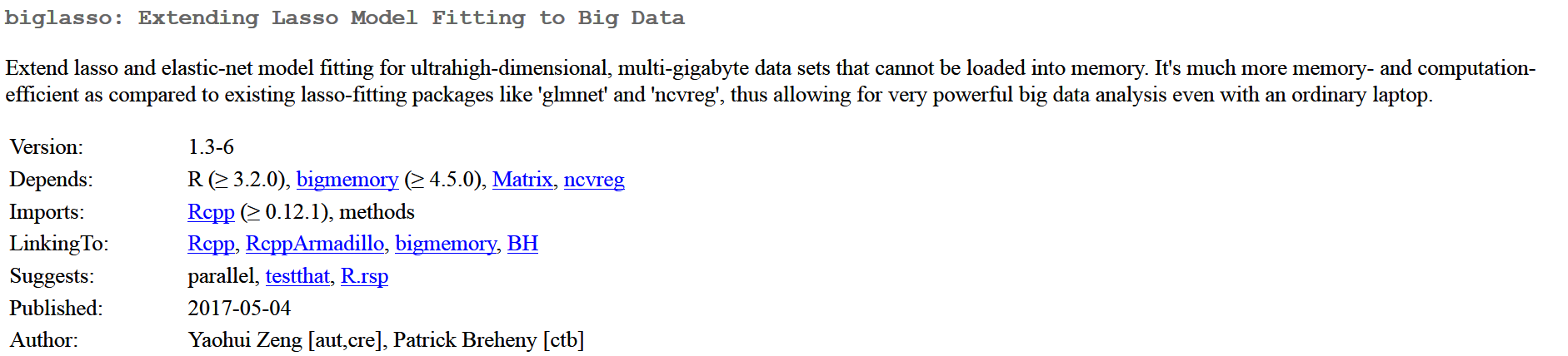
Further packages

# https://cran.rstudio.com/web/packages/biglasso/biglasso.pdf
install.packages("biglasso")

Resources and Links

Myers (1994) Classical and Modern Regression with Applications

Insufficient Solution

Regularized Regression

Regularization

elitedatascience.com definition

Wikipedia definition of Regularization

Strenghts and weaknesses of regularization

Strengths:

Weaknesses:

Three regularized regression algorithms

Lasso regression

Ridge regression

Elastic-net

The objective function of regularized regression methods…

Preparations

Necessary packages

The example dataset

Create training (70%) and test (30%) sets

Ridge Regression

Exemplar coefficients

How to choose the right $\lambda$

Implementation in glmnet

Training and testing feature model matrices and response vectors.

Behind the scenes

A wide range of $\lambda$ parameters

$\lambda$ values in glmnet

Access the coefficients with coef.

Tuning

Results of cv Ridge regression

The plot explained (I)

The plot explained (II)

The plot explained (III)

Coefficients across the $\lambda$ values

Advantages and Disadvantages

Top 25 influential variables

Exercise: ridge regression (I)

Exercise: ridge regression (II)

Exercise: ridge regression (III)

Ridge and Lasso

A Ridge model…

Lasso Regression

Lasso penalty pushes coefficients to zero

The reduction of coefficients

Implementation Lasso regression to ames data

A quick drop in number of features

Tuning with cv.glmnet

MSE for cross validation

Minimum and one standard error MSE and $\lambda$ values.

MSE within one standard error

Model with minimum MSE

Lasso for other models than least squares

Advantages and Disadvantages

Rcode for plotting influential variables

Plot Influential variables

MSE for Ridge and Lasso

Elastic net

Elastic Nets

Summary overview

Implementation

The four model results plottet

Tuning the Elastic Net model

Creation of a tuning grid

Iteration over $\alpha$ values - Elastic Net

The resulting tuning grid

Plot the MSE

MSE +/- one standard error

Predicting

The package caret - Classification and Regression Training

**Vignette for the caret package **

Output for caret model

Which regularization method should we choose?

Advantages and Disadvantages

Further packages

Resources and Links

Links

Implementation in `glmnet`

$\lambda$ values in `glmnet`

Access the coefficients with `coef`.

Tuning with `cv.glmnet`

The package `caret` - Classification and Regression Training

Vignette for the `caret` package

Output for `caret` model